4  Database

4.1 Conventions, in one line each

Names follow Naming conventions: singular lower-case tables, snake_case columns with a unit suffix where one applies, a geom column tagged EPSG:4326, one row per measured value. Keys follow Keys and integrity: a *_key is a string natural key, a *_id an integer, a *_uuid the provider’s own identifier kept as a column; cruise_key, sample_key, site_key/grid_key and taxon_key carry the integration, and every declared key is measured before a release ships.

4.2 The core data model

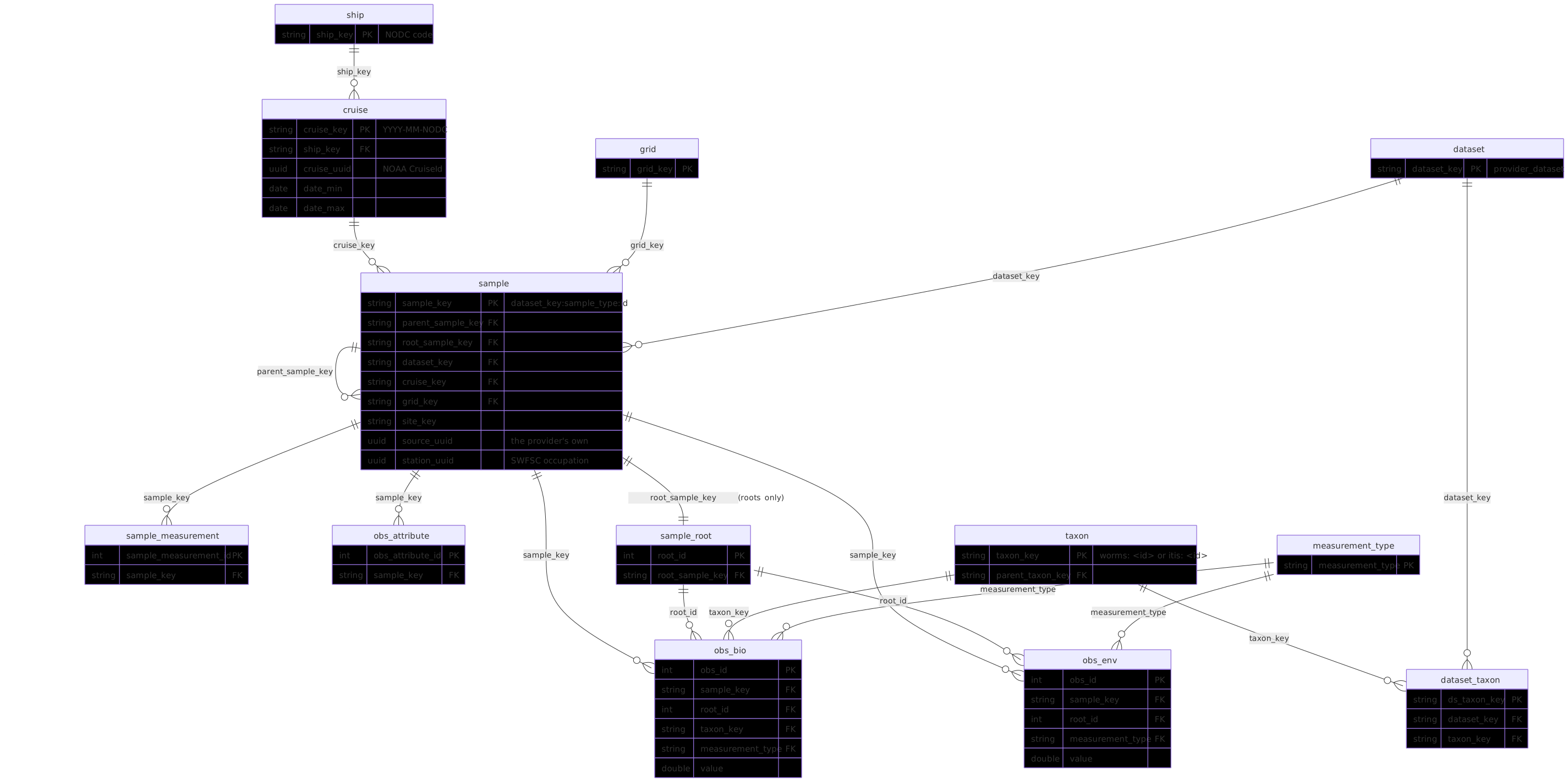
Sixteen source datasets — ichthyoplankton, zooplankton, bottle hydrography, CTD casts, DIC, underway meteorology, seabird and mammal transects, and more — used to reach the database as ~40 per-dataset tables. They now project into a small core family that every consumer reads. A dataset’s projection lives in its own ingest notebook (the generic shapes live in calcofi4db), so adding a dataset never edits a shared switch(). Figure 4.1 draws that family and the reference tables it joins to; Table 4.1 says what one row of each stands for.

Figure 4.1: The core family and the references it joins to, with the keys that carry the integration. Every other released table hangs off one of these; the full diagram for any release is in the schema browser.

Table 4.1: The core family: what one row of each table stands for, and whether it is in the default set.

table	grain	tier
sample	one row per physical sampling event — site, tow, net, cast, bottle, underway record, transect, subsample, region pool — with the hierarchy as an adjacency list (parent_sample_key, plus root_sample_key for the top of the chain)	core
obs_bio	the biological occurrence headline: one scalar per row for a taxon (taxon_key, life_stage, measurement_type, value) with its event’s gear, effort and the two standardized densities inline	core
obs_env	the environmental headline: one measured scalar per row (measurement_type, value, measurement_qual, qual_ok), one parquet object per measurement type	core
obs	the two above under one name — realm = bio or env, value as measurement_value — as a view the catalog carries; its own objects are deprecated	view
obs_attribute	sub-occurrence detail — length- and stage-frequency bins (bin_value, bin_label, count) and categorical behaviour	core
sample_measurement	event-level effort and conditions — a net’s volume_sampled and std_haul_factor, a cast’s surface observations	core
sample_root	one row per root sampling event with the dense integer root_id the browser objects join on, its position, time, depth span, gear and seafloor depth	supplemental
obs_ctd_full	full-resolution CTD scans (~271 M rows); obs_env carries the thinned series	supplemental
obs_mets_full	full-resolution underway meteorology (~20 M rows)	supplemental

Table 4.1 is the whole model in nine rows; Table 4.2 below is every table the release actually ships. An observation’s provenance is denormalized onto it on purpose: obs carries dataset_key, cruise_key, grid_key, the position, the datetime and hex_id (H3 at resolution 10, so coarser aggregations use h3_cell_to_parent(hex_id, res) rather than a column per resolution), so a rollup groups without a join. geom lives on sample and on the reference tables, never on obs.

4.2.1 What the release publishes: obs_bio + obs_env, and obs as a view

The assembly grain is obs; what the release publishes is the pair cut from it, because the questions consumers ask are shaped differently for the two realms:

• obs_bio — one object, the bio realm, with the gear and effort of the row’s own sampling event inline (tow_type, std_haul_factor, prop_sorted, volume_sampled_m3) and the two standardized densities derived once (density_per_10m2, density_per_1000m3) plus effort_class. One taxon question = one file.
• obs_env — one object per measurement_type. One variable = one small fetch, which is what a browser-side reader (DuckDB-WASM cannot list a directory; the catalog gives it an explicit file list) actually needs.

Each is a strict superset of obs under a name mapping — realm is implied by which table you read, and value is measurement_value — and obs itself is a view the catalog carries (catalog.json → views.obs), a UNION ALL over the pair under obs’s original column names. calcofi4r::cc_get_db(), calcofi4py and the query site create it from the catalog, so FROM obs keeps working. Two consequences worth knowing:

• The release proves the pair reproduces obs before it freezes — row counts, distinct obs_ids and a hash signature of every column, per realm × dataset. The one allowed difference is a depth fallback: a bio row with no depth of its own carries its tow’s span.
• obs’s physical objects still ship for one release, marked deprecated in the catalog with replaced_by: ["obs_bio", "obs_env"]. Migrate to the pair — a consumer reading the view needs no change, a consumer building a path to obs.parquet does.

Do not rename value, root_id or hex7 on the pair; new columns are appended and the view maps names, so consumers never have to.

4.2.2 Shared reference tables

cruise (one row per cruise, with cruise_uuid, the ship, and the observed date_min/date_max span that keys every other dataset’s events), ship, grid (the CalCOFI station grid, materialized deterministically from calcofi4r::cc_grid), spatial + spatial_attribute (boundary layers), sample_spatial (the sample→layer memberships), region, lookup, dataset (one row per released dataset, with its measured coverage and its citation), measurement_type (the measurement vocabulary, below) and climatology.

climatology is the one baseline every anomaly subtracts. Until 2026-08-31 three products each computed their own and the same section read +1.4 °C in one and ~0 in another. It is a plain mean per dataset × site_key (the real station, since calcofi4db 4.10.0 — the inshore grid cells hold 2–4 stations 15–30 km apart, so a cell-grained baseline blended them; grid_key stays on the row as the station’s modal cell) × calendar month × 10 m depth bin × measurement type over 1993–2013, kept only where ≥ 5 distinct cruises contribute (3 until v2026.09.06), with the window stamped on every row. A cast’s anomaly is its value minus the row of its own station and calendar month; pooling months produces a seasonal-cycle map, not an anomaly.

4.2.3 Every table in the release

The full inventory — what a database client’s object browser would list — read from the promoted release’s catalog.json and metadata.json. A supplemental table is hosted and catalogued but left out of cc_get_db()’s default set; a deprecated one still ships its objects for one release while its replacement is named.

Table 4.2: Every table of v2026.09.11, with its tier, rows, columns and description.

table	tier	rows	columns	name	description
climatology	core	736,916	12
cruise	core	842	20	Cruise	unique by ship and year-month
dataset	core	16	24	Dataset
dataset_taxon	core	1,917	7	Dataset Taxon	Crosswalk from each dataset’s own taxon vocabulary to the global taxon_key. obs resolves its taxon by joining this on (dataset_key, ds_taxa_code), so a dataset can keep its local codes without leaking them into the shared model.
grid	core	218	10	Grid	CalCOFI survey grid polygons with standard and historical station patterns
lookup	core	26	9	Lookup	Unified vocabulary lookup table for egg stages, larva stages, and tow types
measurement_type	core	200	22	Measurement Type
obs_attribute	core	458,184	10	Observation Attribute	Sub-occurrence attribution: the breakdown within an obs headline row. Covers numeric frequency distributions (length bins, stage numbers) and categorical breakdowns (seabird behavior). Counts here sum to the headline where the source is internally consistent.
obs_bio	core	1,258,665	32
obs_env	core	29,838,093	32
region	core	4	7	Region	The 4 pooled regions defined on the CalCOFI grid (Hayward & Venrick 1998), with the member station codes the source declares and a POLYGON derived from them: each declared station claims the water nearest to it, clipped to the convex hull of all 34 stations and dissolved by region, so the four tile their pooled domain with no overlap and no gaps. Stations are placed by the +proj=calcofi transform rather than a grid lookup, which is what lets the six intermediate inshore stations with no cell in the regularized grid resolve. latitude/longitude is an interior representative point, not a centroid (the regions are concave). Land is not erased. See questions Q01.
sample	core	1,469,151	21	Sample	One row per physical sampling event at its native grain (site, tow, net, cast, bottle, underway, transect, region pool). An adjacency list: parent_sample_key points at the containing event and root_sample_key at the top of the chain, so counting distinct events at any level is a single GROUP BY.
sample_measurement	core	589,603	6	Sample Measurement	Event-level (effort) measurements: quantities that describe the sampling event itself rather than anything observed in it — net volume filtered, standard haul factor, proportion sorted, bottle cast conditions. Kept apart from obs so effort is never mistaken for an observation.
sample_spatial	core	929,632	5
ship	core	49	7	Ship	unique ship with many cruises
spatial	core	13,206	5
spatial_attribute	core	148,461	9
taxon	core	2,614	19	Taxon	Taxonomic hierarchy for species via WoRMS and ITIS authorities (built from spp.duckdb via recursive CTEs)
taxon_group	core	441	3	Taxon Group	Portable groupings of taxa (phytoplankton functional groups, seabirds, marine mammals). Many taxa per group; a taxon may belong to several.
obs	deprecated	31,096,758	18	Observation	The occurrence-headline long table: one scalar measurement per row, environmental (realm = 'env') and biological (realm = 'bio') together. Biological taxon is the global taxon_key; sub-occurrence detail (length/stage bins, behavior) lives in obs_attribute, and event-level effort in sample_measurement.
obs_ctd_full	supplemental	275,231,999	18	Observation (Full CTD)	Supplemental full-resolution CTD scans, identical in shape to obs. Excluded from the default table list and the ERD because of its size; opt in with cc_get_db(supplemental = TRUE). The default obs carries CTD via the adaptively thinned ctd_thin.
obs_mets_full	supplemental	19,926,523	18	Obs Mets Full
sample_root	supplemental	421,450	14

4.2.4 Taxonomy

Three shared tables replace the ~7 per-dataset taxon tables:

• taxon — one row per taxon: taxon_key (worms:<AphiaID>, or itis:<TSN> when the taxon’s class is Aves, because WoRMS bird taxonomy lags), the cross-reference ids (worms_id, itis_id, gbif_id), parent_taxon_key, rank and rank_order, the flattened lineage (kingdom, phylum, class, order_taxon, family), scientific_name, common_name, and taxonomic_status with status_checked — read the two together; a status with no check date is not a fact.
• dataset_taxon — the per-dataset vocabulary → taxon_key crosswalk. obs resolves its taxon_key by joining this on (dataset_key, ds_taxa_code), and ds_source_json records whatever ids the source itself supplied, so the source and the authority can be audited against each other.
• taxon_group — groupings for rollups.

Two distinctions that cost real data before they were written down. The key authority and the cross-reference columns are different questions: a bird keys itis: and carries a worms_id, because a consumer joining on worms_id would otherwise match zero seabirds. And a key must be an accepted id while a cross-reference is whatever the authority links — a deprecated TSN is re-keyed onto its accepted successor and the event is recorded in taxon.notes.

When asserting lineage coverage, split by rank position: family is legitimately NULL above family rank, and kingdom is NULL for worms:1 Biota. A blanket non-NULL assertion is wrong, and someone will “fix” it by inventing data.

4.2.5 A face for every species page

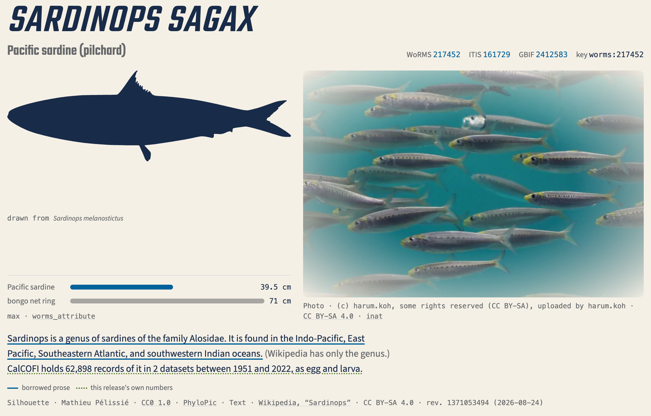
Every taxon has a page at calcofi.io/species/ — the species catalog calcofi4db::build_taxa_catalog() writes as taxa.json, one row per taxon_key with its lineage, authority ids and observation stats. The page also shows a silhouette, a photo where one exists, a size on a familiar scale, and one sentence, so the reader has more than the taxonomy to go on (Figure 4.2). A PhyloPic silhouette, drawn in the page’s own ink, is resolved by WoRMS id and, failing that, by name at each rank up the lineage until one exists. A full-colour photo appears where one clears the licence policy below; where none does, the slot is simply absent and the layout is unchanged. Size is drawn on a scale a reader already knows — the taxon’s own length beside the nearest familiar reference (a US quarter, a person, the CalCOFI bongo net and ring, the ship) — and, for fishes, the egg-to-larva lengths FishBase carries from Matarese et al.’s (1989) laboratory guide of Northeast Pacific early life stages, with CalCOFI Atlas 33 (Moser 1996) held in reserve for the species NOAA’s Ichthyoplankton Information System does not cover. The sentence reuses Wikipedia’s lead under its own licence, followed by the release record’s own numbers. Every source is named on the page: PhyloPic for the silhouette; Wikimedia Commons, iNaturalist and GBIF for the photo; WoRMS, FishBase and SeaLifeBase for the size; NOAA’s Ichthyoplankton Information System for the fish plate. The licence policy is one sentence — Creative Commons and public-domain files are used, non-commercial licences are accepted but labelled, and every asset is credited and linked to its source. None of this is typed into the page: the sidecar (taxa_media.json) is fetched weekly by the landing repo’s own scripts, keyed by taxon_key beside the catalog, and a taxon without a match renders exactly as it does today (taxon-reference skill, Species faces).

Figure 4.2: The page head, composed: a PhyloPic silhouette in the page’s own ink beside a licensed photo faded into the band, a two-bar glance at size against a familiar reference, and a sentence stitched from Wikipedia, the release record and WoRMS, each part underlined in the colour of its source — the Pacific sardine’s live page at calcofi.io, light theme, 2026-09-11.

4.2.6 Measurements

measurement_type.csv names a series — one dataset’s own column of measured values (calcofi_bottle.temperature, calcofi_ctd-cast.temperature_ave). The bottle’s temperature and the CTD’s are the same physical quantity read two ways, and until 2026-09 nothing said so in one place: the Explorer hard-coded five such pairings in its own UNIFIED table with a note that the label “belongs in measurement_type.csv”. The measurements catalog is that one place.

One page per measurement key at calcofi.io/measurements/{key}/ — the registry’s variable where a series belongs to one, else the canonical measurement_type itself — lists every series that measures it, one row per measurement_type × dataset, each with the dataset’s own source and flag column. A series that is not canonical for its key (a raw CTD sensor, a thermosalinograph past the first) gets no page and is listed under its dataset as full_resolution_only[], the vocabulary_only[] of this catalog. This mirrors Taxonomy one-for-one: measurement_type.variable plays dataset_taxon’s crosswalk role, and metadata/variable.csv — read with calcofi4db::read_variable(), appended with register_variables(), never a bare write_csv() — plays taxon’s role of holding the one label, description and NERC P01 concept a key is shown under.

A variable is assigned only where (i) the NERC P01 concept is identical — or the two concepts differ only by a method qualifier for the same quantity — (ii) the units are the same or a declared conversion, (iii) the series come from the same kind of sample, and (iv) the two are not plausibly the same physical samples. calcofi4db::check_variable_registry() enforces (i) and (ii) at write time — a variable.csv row whose nerc_p01 disagrees with a member series’ own value is refused, so a crosswalk key can never silently misdescribe what it unifies. (iii) and (iv) are judgement calls a person records as evidence, not something a function can check from the column alone: the CTD files carry their own embedded bottle table (btl_*) that shares a P01 with the bottle dataset’s series but is plausibly the same physical bottles measured twice, so it fails (iv) and stays its own key, related to the bottle’s on each page with the reason (same_bottles); a replicate is not a mean (replicate_vs_mean); an underway intake is not a cast (underway_vs_cast). Table 4.3 is every key variable.csv carries on v2026.09.11, with its member series — sigma_theta’s two series keep their own NERC concepts (the bottle’s by computation, the CTD’s by CTD and computation) because criterion (i) reads “or a method qualifier,” not “identical always.”

The record, measurements.json (calcofi4db::build_measurements_catalog(), schema measurements.schema.json, written beside taxa.json in release_database.qmd), is taxa.json‘s twin for the environment half of the catalog: counts, one datasets[] entry per dataset carrying an obs_env row, one measurements[] entry per key with series[] carrying each series’ values by year, month, depth band and quality code, the observed quantiles within the registry’s declared bounds, and related[] naming the other keys that share a NERC P01 concept and are kept apart on purpose. test_release.qmd’s measurements_catalog gate re-derives the schema check and the arithmetic gate every consumer of this record leans on: the sum of series[].n_values over every key equals obs_env’s own row count, which is exactly what a series counted into two keys would break.

On v2026.09.11, the record (release) counts 89 measurements over 94 series in 5 datasets — 29,838,093 obs_env rows, 324,996,615 once the two full-resolution supplementals are counted.

Table 4.3: Every unified measurement key on the record above, with its member series — the dataset, the series’ own column, its values, and its own NERC P01 concept (identical for four keys; sigma_theta’s differ by method qualifier, D3 criterion i).

	series (column)	values	NERC P01
Dissolved oxygen (ml/L)
calcofi_bottle	oxygen_ml_l	725,629	DOXYZZXX
calcofi_ctd-cast	oxygen_ml_l_ave_sta_corr	653,231	DOXYZZXX
Dissolved oxygen (µmol/kg)
calcofi_bottle	oxygen_umol_kg	690,697	DOXMZZXX
calcofi_ctd-cast	oxygen_umol_kg_ave_sta_corr	626,394	DOXMZZXX
Salinity
calcofi_bottle	salinity	848,013	PSLTZZ01
calcofi_ctd-cast	salinity_ave_corr	673,276	PSLTZZ01
Potential density (σθ)
calcofi_bottle	sigma_theta	842,669	SIGTEQ01
calcofi_ctd-cast	sigma_theta_1	690,881	SIGTPR01
Temperature
calcofi_bottle	temperature	884,400	TEMPPR01
calcofi_ctd-cast	temperature_ave	691,159	TEMPPR01

Two facts the record states rather than leaves implicit. A series with no NERC concept says so — no_p01 on its flags, never a blank cell that reads as “not looked at” — the same exact-match discipline as every controlled-vocabulary id in Metadata registries: 38 of the 94 series on v2026.09.11 carry no P01. And a bound is declared or questioned, never inferred from the data (the ingest’s own rule — measurement bounds): a series’ observed{} range is computed within its registry bound, what falls outside is counted separately in out_of_bounds{n, min, max} rather than silently widening the range a reader sees, and 15 series declare no bound at all (no_bound) rather than letting their widest reading stand in for one; 2 series carry sentinel_suspected — a declared bound broken, or, absent one, an extreme past ±99 and 100× the series’ own 5th/95th percentile. That is how the catalog surfaced a sea-surface reading of thousands of degrees and a PAR sensor’s numeric fill value on v2026.09.11 — both certain bugs, fixed at the ingest, not questions. ### A face for every measurement page

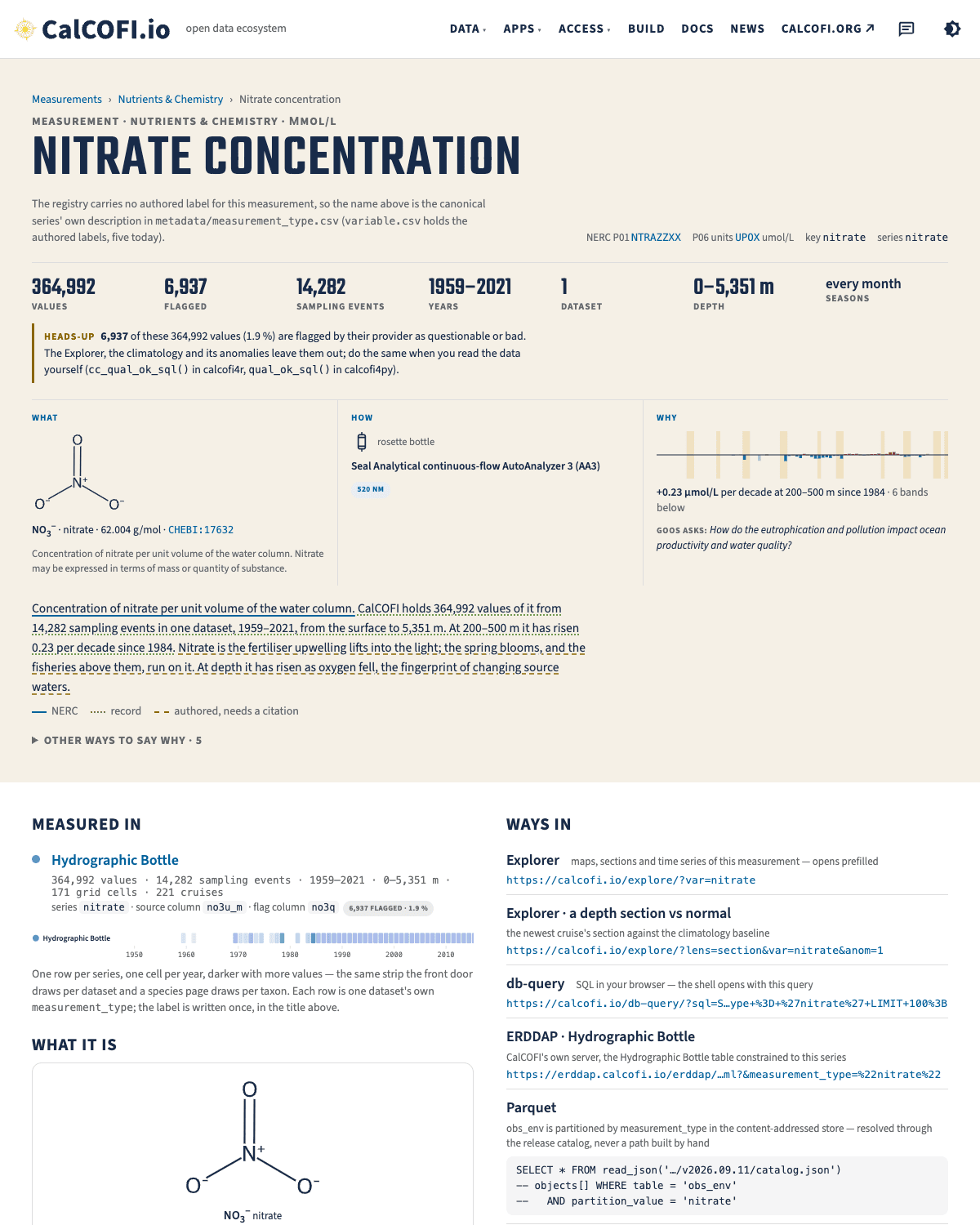
Every measurement page at calcofi.io/measurements/{key}/ carries the catalog above, and beneath it a face that answers three questions in one glance: what the thing is, how CalCOFI takes it, and why it matters (Figure 4.3). What follows NERC’s own identity chain — a P01 concept’s sameAs link to a chemical entity in ChEBI, or a biological one in WoRMS — down to a structure drawn from ChEBI’s own coordinates, in the page’s own ink; a mixture such as salinity shows its composition instead, the mass fractions of TEOS-10’s Reference-Composition Salinity Scale (Millero et al. 2008) rather than a single molecule, and a property with no chemical identity of its own shows its familiar scale alone. How comes from metadata/measurement_method.csv, one row per dataset and measurement key naming the platform, the instrument, the principle, and a link into the method’s own section of calcofi.org, styled like the front door’s pins. Why is one sentence stitched from the NERC definition, the release record’s own anomaly for every depth band where the quantity is measured against its climatology, and a single authored, cited line picked as the best one-sentence answer; the alternatives not picked — a second authored line, the GOOS essential-ocean-variable question, the Wikipedia lead — wait one click away in a collapsed panel, the same idiom the datasets catalog uses for what is “not yet in the database.” A key with no NERC concept of its own — an instrument voltage, an estimate, a sensor pair’s average — borrows the face of the quantity it stands in for and says so on the page, rather than showing a face for a concept it does not carry. None of this is typed into the page: the sidecar (measurements_media.json) is fetched by the landing repo’s own scripts, keyed by measurement key beside the catalog, and a key without media renders exactly as it does today (metadata-registries skill, Measurement faces).

Figure 4.3: The page head, composed: the existing crumb, label, NERC ids and stats band, with a new face row beneath it — a molecule drawn from ChEBI’s own coordinates in the page’s own ink, a link to the method on calcofi.org, and a sentence stitched from the NERC definition, the release record and an authored, cited line, each part underlined in the colour of its source — the live nitrate page at calcofi.io, light theme, 2026-09-12.

4.2.7 Quality flags reach consumers only if consumers apply them

obs.measurement_qual is each dataset’s own vocabulary, uninterpreted — bottle 6 = ok-from-CTD, 8 = suspect, 9 = missing; CTD 1/2 = use primary/secondary sensor, 8 = questionable, 9 = bad; DIC follows WOCE (2 good, 3 questionable, 4 bad, 9 missing). The registry is metadata/measurement_qual.csv in the workflows repo and it ships in metadata.json.

In August 2026 a 2.18 ml/L oxygen spike at 1,144 m turned out to be a bottle flagged suspect in the source since 1955 — it reached a plotted app because no consumer filtered on the column. There is now one predicate per language — calcofi4r::cc_qual_ok_sql(), calcofi4py.qual_ok_sql(), the query site’s qualOkSQL() — NULL-safe, so an unflagged row is kept. Apply it. A value with a flag you do not read is not a value you can trust.

4.2.8 Depth is a coordinate, and it is bounded as one

Every released depth is finite, non-negative and no deeper than 6,500 m, on obs, on sample and on the supplemental tables; a violation fails the release rather than shipping. Separately, sample.seafloor_depth_m carries the GEBCO 2025 sea-floor depth at the sample’s position (positive down, 0 on land, NULL outside the raster) so a consumer can judge a deep sample without fetching a raster. Where a sample’s deepest attributed depth exceeds the deepest GEBCO cell near it, that is reported and ratcheted, never deleted: nearly all such cases are minute-rounded 1949–1975 positions on slopes and canyons — the measurement is fine, the place is imprecise.

4.3 Integrated database ingestion strategy

4.3.1 Overview

The integrated database is built by the CalCOFI/workflows pipeline: one ingest_{provider}_{dataset}.qmd notebook per dataset (orchestrated by targets, engine functions in calcofi4db) writes Parquet shards plus JSON sidecars; release_database.qmd assembles them in an in-memory DuckDB, validates, and freezes a versioned, immutable release on public Google Cloud Storage (next section). Consumers — the apps, calcofi4r::cc_get_db(), the schema and query sites — read the release as Parquet over HTTPS with no credentials.

Alongside the releases stands a PostgreSQL database (calcofi, PostgreSQL 18 + PostGIS 3.6 on the CalCOFI server) built as a working, multi-user store for the CTD team’s QA/QC: originals loaded verbatim and immutable, a flag/proposal ledger beside them, derived products on top. It is available but not yet adopted — the team’s flags still arrive with the provider’s files — and no part of the pipeline reads it live in either case; the bridge is a nightly parquet snapshot (CTD QA/QC). It is private and reached over SSH — see Server Access. DuckDB’s postgres extension joins the two worlds in one query (calcofi4r::cc_pg_attach()). (An earlier design ran the whole database in PostgreSQL with dev/prod schemas and a single create_db.qmd; that is superseded and only the legacy gis database remains, behind tile.calcofi.io.)

4.3.2 Release versioning

A release is an immutable, versioned copy of every table under gs://calcofi-db/ducklake/releases/{version}/, described by its catalog.json, content-addressed, with a DOI per version and one concept DOI for all of them. What ships, which versions are kept, how to pin one and what is checked before a release is cut are in Releases.

4.3.3 Metadata registries — the single sources of truth

Descriptions, vocabularies and provenance live as reviewable CSVs in CalCOFI/workflows — not in the database — so they travel with the code that produced them and change through pull requests.

Per dataset, under metadata/{provider}/{dataset}/:

• tbls_redefine.csv — tbl_new, tbl_description
• flds_redefine.csv — the crosswalk from every source column to its standard name and type (Naming conventions)
• metadata_derived.csv — optional markdown/units overlay for derived tables and columns
• questions.csv — the provider-question registry: what we have asked the data’s owners, what they answered, and what we have proposed an answer to and want confirmed. Each question has a durable global id and a short per-dataset label (Q15), a status (open / proposed / answered / wontfix) and a priority.
• dataset_meta.yml — the descriptive half of the dataset’s metadata: abstract, methods, creators, citation, licence, DOI, contact, keywords (Metadata & the ingest loop)
• citation_authority.json — a generated cache of what the source’s own authority (EDI, NCEI, ERDDAP, DataCite) says about the citation and licence. A proposal, never the record.

Shared, under metadata/:

Table 4.4: The shared registries under metadata/ in CalCOFI/workflows, and what each is the record of.

file	role
field_dictionary.csv	Prescriptive canonical field names, types, units and aliases; new datasets conform to it. dwc_term names the Darwin Core term a field publishes as.
measurement_type.csv	The canonical measurement vocabulary — description, units, category, variable (which types measure the same thing comparably across datasets), derivation for a derived type, is_canonical, the validity bounds, and the controlled-vocabulary ids nerc_p01 / units_nerc_p06 (below). Released as a table.
variable.csv	One row per crosswalk key measurement_type.variable points at (D3, Measurements) — its label, description, units, category and NERC P01, held once for the key rather than repeated on each member series. Read with read_variable(), appended with register_variables(), checked against measurement_type.csv with check_variable_registry().
measurement_qual.csv	Each dataset’s quality-flag vocabulary, uninterpreted.
category.csv	The twelve data categories every dataset and measurement type is filed under.
provider.csv	The curating organizations. provider is the organization that holds and can license the data — not the portal that serves it, and not a collection or lab inside it.
license.csv	The licence ids a dataset may declare.
life_stage.csv	Every distinct obs.life_stage value with its Darwin Core label and NERC S11 id.
gear.csv	Every sample.tow_type code with its samplingProtocol sentence and NERC L22 device id.
dataset_meta_fields.csv	The tiers of authored dataset metadata (required, recommended, optional) and the guidance a provider sees for each; the field list every dataset_meta.yml follows.
dataset_status.csv	The pipeline-stage tracker, one row per dataset, and each dataset’s archive-of-record policy sentence.
distribution.csv	Every curated endpoint per dataset the release cannot measure itself — mirrors, archive records, the OBIS dataset, legacy ERDDAP ids with their successors — never deleted, only statused.
distribution_observed.json	Generated weekly: what each portal says now about every distribution; a change files a proposed provider question, never an edit.
portal.csv	The portals themselves — what each holds, how it can be queried, what it harvests from calcofi.io (Portals).
holdings.csv	Generated at release: the datasets CalCOFI holds but has not ingested, from their sidecars.
taxon_group.csv	The rules that assign taxa to the groups the apps offer (functional groups, “other”); a group label never becomes a taxon’s common name.
questions_sheets.yml	Which Google Sheet each provider’s questions and metadata tabs live in (Metadata & the ingest loop).
relationships_cross.csv	Cross-dataset foreign keys (intra-dataset ones live in each ingest’s relationships.json); every edge is measured at release (Keys and integrity).
release_tables.csv, release_columns.csv	Descriptions for tables built inside release_database.qmd itself.
measurement_taxon.csv, taxon_override.csv	How a taxon-bearing measurement name decomposes, and manual id resolution where a source taxon has no clean id.
taxon_lineage.csv, taxon_xref.csv	Generated caches of the WoRMS/ITIS classification chains and the WoRMS↔︎ITIS cross-reference. Safe to delete; they refetch.
dataset.csv	Deprecated. A dataset’s structural keys are the calcofi: YAML block in its ingest notebook; its descriptive metadata (abstract, citation, license, DOI, contact, …) is the metadata/{provider}/{dataset}/dataset_meta.yml sidecar, and the release reads the two merged (see Metadata & the ingest loop and Cite This Data). The CSV drifted from the notebooks and orphaned observations.

The per-dataset files above and the shared registries of Table 4.4 flow through two stages:

1. Per ingest: calcofi4db::build_metadata_json() writes data/parquet/{provider}_{dataset}/metadata.json (schema version 1.0) beside the parquet outputs, and reports its own documentation gaps.

2. Per release: calcofi4db::merge_metadata_json() merges every per-ingest sidecar plus the release-only registries into gs://calcofi-db/ducklake/releases/{version}/metadata.json (schema version 1.2):

   {
     "schema_version": "1.2",
     "release_version": "v2026.09.06",
     "release_date":    "2026-09-06",
     "datasets":          { "calcofi_bottle": { ... } },
     "tables":            { "sample":  { "name_long": "Sample",
                                         "description_md": "One row per physical sampling event …",
                                         "provider": "swfsc", "dataset": "ichthyo" } },
     "columns":           { "sample.depth_min_m": { "name_long": "Depth Min",
                                                    "units": "m",
                                                    "data_type": "DOUBLE",
                                                    "description_md": "Shallowest depth of the event" } },
     "measurement_types": { "temperature": { "description": "...", "units": "degC",
                                             "is_canonical": true } },
     "contributions":     { "sample": { "swfsc_ichthyo": 0.62, "calcofi_bottle": 0.31 } },
     "erd_legend":        [ { "provider_dataset": "calcofi_bottle", "color": "#f5cad9" } ]
   }

contributions is each dataset’s share of a shared table’s rows (the bar on a schema-browser card); erd_legend the colour each dataset takes in the diagram.

Markdown is supported anywhere in description_md; consumers should render it through a markdown parser when displaying.

4.3.4 Coverage is measured, never asserted

A dataset’s temporal and spatial extent is measured from the assembled data at release time — coverage_temporal_observed, coverage_spatial_observed and coverage_bbox in metadata.json, and coverage_temporal / coverage_spatial on the released dataset table (the measured values, under the plain names). Nothing hand-writes an extent.

This is not pedantry. A hand-written extent is authored once while the data grows underneath it: at v2026.08.06 seven of fifteen datasets were wrong — one claimed data through 2021-05 that ends 2015-04, three said “present” while stalling in 2019, 2022 and 2023. Measurement is also honest about what it finds, which is how two coordinate bugs surfaced that the prose had hidden (a dropped minus sign putting a dataset at 124.9° E, and a dataset reaching latitude 0.0). One dataset asserts its temporal half and says why in a comment: it is region-pooled and has no datetimes at all.

4.3.5 Citation and licence are a contract, and they are checked

Every dataset carries citation_main, license, doi, acknowledgement and contact in its dataset_meta.yml sidecar, and these are checked, not trusted — by the workflows index build and again by the release. A citation needs a year and a locator; license must be an active id in license.csv (custom requires a license_url; unknown or empty fails unless a provider question is open on that field); a doi is stored bare and must resolve. The check also asks the source’s own authority — EDI’s cite service, NCEI’s “Cite as”, an ERDDAP .das, DataCite — caches the answer, and reports drift without ever writing into the notebook: the author’s string is the record.

source_accessed is measured, not authored. And the release cites itself: catalog.json carries a citation, a concept_doi and, once minted, the version doi; the release notes open with “How to cite”; CITATION.cff and .zenodo.json are generated from the same source.

CalCOFI (2026). CalCOFI Integrated Database, release v2026.09.06 [Data set].
Scripps Institution of Oceanography, NOAA Fisheries, and California Department
of Fish and Wildlife. https://doi.org/10.5281/zenodo.22514953

(That is the release promoted as this page was written; the current one is in catalog.json and on Cite This Data.)

When you use these data, cite the release and the source datasets you used. The release dataset table carries each source’s own citation_main, license, doi and acknowledgement for exactly this purpose — one row per dataset, so a query that touched dataset_key already knows whom to credit.

4.3.6 Consuming descriptions

The fastest way to browse the schema is the CalCOFI Schema explorer — per-release ERD, sortable table/column lists with units, dataset provenance, and the measurement-type registry, all sourced from the release metadata.json sidecar on GCS. Deep-link to a specific release with #erd?v=v2026.08.25 (or #tables, #columns, #measurements).

From R, fetch the descriptions either column-by-column or as a full interactive catalog. Both calls hit the same release metadata.json sidecar:

library(calcofi4r)

# schema + descriptions + units for a single table
tbl <- cc_describe_table("sample")
attr(tbl, "description_md")    # table-level description

# interactive datatable of every table and column in the release
cc_db_catalog()
cc_db_catalog(tables = c("sample", "obs_bio"))
cc_db_catalog(version = "v2026.08.25")

When writing a new ingest, populate tbls_redefine.csv and flds_redefine.csv (especially fld_description and units) before running the ingest notebook — build_metadata_json() reads them directly. The Claude Code /generate-metadata and /validate-ingest skills enforce this.

4.3.7 Publishing to portals

Workflows in workflows/publish_to-*.qmd push selected tables to external portals — ERDDAP, EDI, OBIS — and write netCDF for the archives. They read the release catalog.json and metadata.json to assemble Ecological Metadata Language (EML), ERDDAP datasets.xml entries and netCDF attributes, so a description written once in a metadata registry reaches every portal without re-keying, and so no publish notebook builds a parquet path by hand.

The netCDF, ERDDAP, EDI and OBIS publishers are all generic — parameterised by dataset, driven by the release; the OBIS one (publish_to-obis.qmd, 2026-09-05) retired the per-dataset ichthyoplankton notebook. See Darwin Core / OBIS ENV-DATA mapping for what it reads, and Portals for the publishing steps. All four run after every promoted release and rebuild a dataset’s output only when its rows, metadata or the publisher’s code changed; publish_status.qmd then lists which portal copies are due a fresh upload (Portals).

ERDDAP (publish_to-erddap.qmd) discovers one config block per dataset_key from what the core actually holds, rather than a hand-maintained table list, and executes every view against the real release before writing its XML. Since the pre-release plan D-S1/D-S3 (2026-09) the {dataset_key} observation grain reads obs_bio (bio datasets) or obs_env (env datasets) through the release catalog (calcofi4r::cc_release_sources()) — never a hand-built releases/{v}/parquet path — carrying the sample’s own gear and effort (tow_type, std_haul_factor, prop_sorted, volume_sampled_m3) and the two canonical densities (density_per_10m2, density_per_1000m3, effort_class) inline, plus flag_values/flag_meanings on measurement_qual from metadata/measurement_qual.csv. A release cut before D-S1 (no obs_bio/obs_env in its catalog) falls back to the deprecated obs objects, with no effort/density columns.

4.4 Darwin Core / OBIS ENV-DATA mapping

The core model was designed against the OBIS ENV-DATA pattern described by De Pooter et al. (2017), so the shapes map one to one: sample’s adjacency list is an Event core, obs’s bio rows are an Occurrence extension, and the two measurement grains are extended Measurement-or-Fact tables. What was missing was never the shape — it was the vocabulary: an export had to guess which controlled term a CalCOFI measurement name meant, and the ichthyoplankton OBIS notebook did not guess, it wrote measurementTypeID = NA.

The ids now live in the registries the release already publishes, so a portal export is a lookup rather than a judgement.

Table 4.5: How each core table publishes as Darwin Core under the OBIS ENV-DATA pattern.

CalCOFI	Darwin Core / OBIS ENV-DATA	how it is constructed
sample (adjacency list)	Event core	eventID = sample_key; parentEventID = parent_sample_key; eventDate from datetime (a tow publishes as its start/end interval); decimalLatitude / decimalLongitude; minimumDepthInMeters / maximumDepthInMeters = depth_min_m / depth_max_m; footprintWKT from geom; locationID = site_key; samplingProtocol from metadata/gear.csv keyed on tow_type; sampleSizeValue = volume_sampled_m3 with sampleSizeUnit = cubic metre
obs_bio (obs where realm = 'bio')	Occurrence extension	occurrenceID from obs_id; eventID = sample_key; scientificNameID built from taxon_key (urn:lsid:marinespecies.org:taxname:<worms_id>, or the ITIS TSN for a bird); scientificName from taxon; lifeStage + its NERC S11 id from metadata/life_stage.csv; organismQuantity = density_per_10m2 or density_per_1000m3 with organismQuantityType naming that denominator
sample_measurement	eMoF on Events (net effort, cast conditions)	measurementType / measurementValue / measurementUnit, plus measurementTypeID = measurement_type.nerc_p01 and measurementUnitID = measurement_type.units_nerc_p06
obs_attribute	eMoF on Occurrences (length and stage frequency)	bin_value / bin_label / count → measurementValue; ids as above
obs_env (obs where realm = 'env')	eMoF on the bottle or depth Event	ids as above

Every row of Table 4.5 is a lookup in a registry the release already publishes, not a judgement made at export time. metadata/field_dictionary.csv carries a dwc_term column holding the full term URI for the 12 of 57 canonical fields that one Darwin Core term means exactly. A field Darwin Core splits — depth_m becomes minimumDepthInMeters and maximumDepthInMeters — or has no term for is deliberately left empty rather than mapped approximately.

4.4.1 An id is filled only on an exact match

Empty means “no concept in the vocabulary says exactly this”, never “nobody looked.” An id is written only when every facet the concept states — quantity, matrix, phase, method — is something the registry or the dataset’s documented protocol actually supplies. A generic concept is an exact match at coarser specificity: NERC P01 TEMPPR01, Temperature of the water body, is exactly what a QC’d bottle temperature is. A concept that adds a facet nobody recorded is not: IRRDUV01 pins PAR to a cosine-collector radiometer, which no CalCOFI metadata states, so PAR has no id.

Filling an id you are not sure of is worse than leaving it empty. An empty measurementTypeID is a portal record that says “this measurement is not mapped”; a wrong one is a record that confidently says the wrong thing, at an aggregator that will never ask.

Coverage as of v2026.09:

Table 4.6: Controlled-vocabulary coverage per registry — filled only on an exact match.

registry	column	filled
measurement_type.csv	nerc_p01 (P01, measurementTypeID)	115 / 200
measurement_type.csv	units_nerc_p06 (P06, measurementUnitID)	174 / 200
life_stage.csv	nerc_s11 (S11, lifeStage)	10 / 23
gear.csv	nerc_l22 (L22, samplingProtocol device)	4 / 11
field_dictionary.csv	dwc_term	12 / 57

The gaps in Table 4.6 are deliberate, and mostly not gaps. Of the 85 measurement types with no P01, 29 are taxon-bearing abundance, biomass or size types — P01 encodes the taxon in the concept, and CalCOFI carries it in taxon_key, so a per-type id there would be wrong rather than missing. Another 8 are event-level effort and sub-occurrence attributes BODC does not model as parameters. The genuine gaps are documented in RELEASES.md, and most of them are questions for a data provider rather than for the vocabulary: an unrecorded transmissometer wavelength, radiation channels that do not say whether they are upwelling or downwelling, flow-cytometry gating that was never written down.

4.4.2 Three caveats for anyone building an export

• obs is positive-only for ichthyoplankton. A tow that was sorted and found nothing has no row, so occurrenceStatus = "absent" cannot be derived from zero values. Absences come from the sampling events (sample, root rows) minus the taxa observed on them — and a surveyed year with no positives is indistinguishable from an unsurveyed year if you count rows instead of events.
• organismQuantityType is the whole meaning of the number. Areal (individuals per 10 m², from an oblique or vertical tow standardized by the haul factor) and volumetric (individuals per 1000 m³, from a surface Manta tow or any tow with a filtered volume) are not interconvertible without an integrated depth and a vertical-distribution assumption. Publish the denominator with the number, never a bare count.
• Two life_stage values are not life stages. Euphausiid damaged marks specimens too damaged to stage (occurrenceRemarks), and ichthyoplankton invert is a provenance flag for the merged invertebrate counts. metadata/life_stage.csv says so per value; do not pass either through as lifeStage.

The generic publish_to-obis.qmd over the core reads exactly these registries; it replaced the per-dataset ichthyoplankton notebook on 2026-09-05 (see Portals).

4.5 Relationships between tables

Primary and foreign keys ship with every release as relationships.json beside catalog.json, and since 2026-09-08 every one of them is measured before the release is cut and the result ships as integrity.json. The keys, the joins worth memorising and the measured result are in Keys and integrity; the schema browser draws the diagram per release.

4.6 Spatial Tips

• Use ST_Subdivide() when running spatial joins on large polygons.

• All released geometry is tagged EPSG:4326, normalized immediately before the freeze. This matters because ST_Point(lon, lat) tags OGC:CRS84 while ST_Read() over GeoJSON tags EPSG:4326 — the same WGS 84 longitude/latitude — and DuckDB refuses ST_Intersects across differing tags. If you build geometry on one side of a join, tag both sides; do not coerce one to match the other, or the next release will break you.

• NaN is not NULL, and it corrupts spatial queries beyond its own row. A NaN coordinate survives IS NOT NULL, and ST_Point(NaN, NaN) returns a real, non-NULL geometry that survives geom IS NOT NULL too. Worse, its presence makes ST_Intersects return different counts at different thread counts, dropping valid, unrelated pairs. The release normalizes NaN/Inf to NULL before minting geometry — but if you build your own, test isnan() and isinf() explicitly.

De Pooter, Daphnis, Ward Appeltans, Nicolas Bailly, Sky Bristol, Klaas Deneudt, Menashè Eliezer, Ei Fujioka, et al. 2017. “Toward a New Data Standard for Combined Marine Biological and Environmental Datasets — Expanding OBIS Beyond Species Occurrences.” Biodiversity Data Journal 5: e10989. https://doi.org/10.3897/BDJ.5.e10989.

Matarese, Ann C., Arthur W. Kendall, Deborah M. Blood, and Beverly M. Vinter. 1989. “Laboratory Guide to Early Life History Stages of Northeast Pacific Fishes.” NOAA Technical Report NMFS 80. National Oceanic; Atmospheric Administration, National Marine Fisheries Service. https://spo.nmfs.noaa.gov/sites/default/files/legacy-pdfs/tr80.pdf.

Millero, Frank J., Rainer Feistel, Daniel G. Wright, and Trevor J. McDougall. 2008. “The Composition of Standard Seawater and the Definition of the Reference-Composition Salinity Scale.” Deep-Sea Research Part I: Oceanographic Research Papers 55 (1): 50–72. https://doi.org/10.1016/j.dsr.2007.10.001.

Moser, H. Geoffrey, ed. 1996. The Early Stages of Fishes in the California Current Region. CalCOFI Atlas 33. California Cooperative Oceanic Fisheries Investigations. https://calcofi.org/downloads/publications/atlases/CalCOFI_Atlas_33.pdf.