Summer CTD temperature anomalies against a 1993-2013 baseline • calcofi4r

What this shows

A complete anomaly analysis using five calcofi4r functions — cc_transect_stations(), cc_transect_section(), cc_climatology(), cc_anomaly() and cc_transect_matrix() — against the public CalCOFI release, with no credentials and no SQL.

The worked question is a real one, from Rasmus Swalethorp (SIO) for a CCIEA workgroup: extract the summer cruise temperature data and generate anomaly plots using 1993–2013 as the baseline.

1993–2013 is newly possible. Until the August 2026 release the 1 m-binned CTD record jumped straight from 1998 to 2003 — calcofi.org publishes Final 1 m-binned products for 1998 and 2003 onward, and only raw cast files before that. A backfill from Jim Wilkinson’s archive closed the gap, so that baseline now means what it says instead of quietly meaning “1998, plus 2003–2013”. The last section quantifies what the difference is worth.

library(calcofi4r)
library(dplyr)
library(ggplot2)
library(tidyr)

con <- cc_get_db()

Parameters, stated once

The choice of baseline is the single assumption a reader of an anomaly plot most needs to see, so it lives at the top rather than inside a call.

BASELINE  <- c(1993, 2013)   # inclusive
SUMMER    <- 7:8             # CalCOFI's summer occupation runs Jul-Aug
LINE      <- 93.3            # the line off San Diego; every core line works
VAR       <- "temperature_ave"
DEPTH_MAX <- 500
MIN_N     <- 3               # baseline cells thinner than this are dropped

One transect

A transect here is one CalCOFI line, ordered by station number ascending — nearshore to offshore. There are no endpoints to pick, which is what makes any line × cruise drawable without user input. It is deliberately not the order stations were occupied: that is the ship’s track, so its direction is whichever way the ship steamed, and it is missing on roughly half the release’s cast rows.

cruises <- tbl(con, "sample") |>
  filter(dataset_key == "calcofi_ctd-cast", sample_type == "cast") |>
  mutate(yr = as.integer(strftime(datetime, "%Y")),
         mo = as.integer(strftime(datetime, "%m"))) |>
  count(cruise_key, yr, mo, data_stage, name = "n_casts") |>
  collect()

summer <- filter(cruises, mo %in% SUMMER)
cruise_recent <- summer |> filter(yr == max(yr)) |> slice(1) |> pull(cruise_key)

sta <- cc_transect_stations(con, LINE, cruise_recent)
sec <- cc_transect_section(
  con, LINE, cruise_recent, variables = VAR, depth_max = DEPTH_MAX)

head(sec)
#> # A tibble: 0 × 6
#> # ℹ 6 variables: cruise_key <chr>, sta <dbl>, dist_km <dbl>, depth_m <dbl>,
#> #   variable <chr>, value <dbl>

cc_transect_stations() also decides the horizontal ruler. x = "occupied" (the default) measures between the stations this cruise actually occupied, so the section fills the plot; x = "line" measures along the full line, so cruises covering different extents are comparable in width.

That is not cosmetic. Line 93.3 has not been sampled past station 90 since January 2025, though 113 of the 130 cruises before that reached station 120:

occ <- cc_transect_stations(con, LINE, cruise_recent, x = "occupied")
lin <- cc_transect_stations(con, LINE, cruise_recent, x = "line")

c(occupied_km = max(occ$dist_km), along_line_km = max(lin$dist_km))
#>   occupied_km along_line_km 
#>      468.7072      470.4013

The baseline, and a filter before it

clim <- cc_climatology(
  con, variables = VAR, years = BASELINE, depth_max = DEPTH_MAX, min_n = MIN_N)

attr(clim, "baseline")
#> [1] 1993 2013
nrow(clim)
#> [1] 34558

cc_climatology() is a plain mean per (station, 5 m depth bin, calendar month) — the finest grouping CalCOFI’s design supports, since quarterly-ish cruises over decades give many years per calendar month at a station but only a handful of days. It returns clim_n so a thin cell is visible rather than silently trusted.

Screen the source for physically impossible values

Do this before computing a baseline, not after looking at the result. The released CTD carries a small number of surface readings that are not ocean temperatures — the classic soak artifact, where the sensor is still warm from sitting on deck and has not equilibrated in the first metre or two of the downcast.

There are only 18 such rows in 13.5 million, and the release’s declared bounds (−2 to 40 °C, deliberately set to “impossible” rather than “unusual”) let them through. But they land in the sparsely-sampled northern lines, where an April baseline cell may hold only 2–7 observations in the entire 1993–2013 window — so one 38 °C reading moves that cell’s mean by more than 10 °C, and every other April cruise at that station then reads as a spurious ~11 °C cold anomaly.

The data makes the cut obvious: there is nothing at all between 26 and 35 °C.

temp_all <- tbl(con, "obs") |>
  filter(dataset_key == "calcofi_ctd-cast", measurement_type == VAR,
         !is.na(measurement_value)) |>
  select(measurement_value, depth_min_m) |>
  collect()

temp_all |>
  mutate(band = cut(measurement_value, c(-Inf, 24, 26, 30, 35, Inf),
                    labels = c("<24", "24-26", "26-30", "30-35", ">=35"))) |>
  count(band)
#> # A tibble: 3 × 2
#>   band       n
#>   <fct>  <int>
#> 1 <24   652202
#> 2 24-26      1
#> 3 >=35      18

So a regional ceiling well inside that gap removes every artifact and nothing else. This is a client-side screen — the release keeps the rows, and the values are reported to the data provider as Q22 so they can be fixed at source rather than papered over by every downstream user in their own way.

# Two-sided, on purpose. An earlier draft screened only the upper bound, because
# the artifact I had in front of me was a hot one — which would have sailed past
# the cold artifact that motivated this whole exercise (a failed sensor averaged
# into TempAve produced values near -47 degC). A screen that can only catch the
# failure you already know about is not a screen.
#
# 0 and 30 degC: roughly 5 degC outside the coldest and warmest genuine CalCOFI
# readings, and far outside anything the region produces. Nothing legitimate is
# near either bound.
TEMP_RANGE_REGIONAL <- c(0, 30)

screen <- function(d, col = "measurement_value")
  filter(d, .data[[col]] >= TEMP_RANGE_REGIONAL[1],
            .data[[col]] <= TEMP_RANGE_REGIONAL[2])

clim_screened <- cc_climatology(
  con, variables = VAR, years = BASELINE,
  depth_max = DEPTH_MAX, min_n = MIN_N) |>
  filter(clim_mean >= TEMP_RANGE_REGIONAL[1],
         clim_mean <= TEMP_RANGE_REGIONAL[2])

nrow(clim) - nrow(clim_screened)   # baseline cells the screen removes
#> [1] 1

Anomalies for one section

cc_anomaly() differences a section against the climatology, matched on station, calendar month and depth bin. A cell with no baseline comes back NA, never 0 — an unsampled baseline is not a zero anomaly, and collapsing the two is how a plot ends up colouring “normal” somewhere never measured.

anom <- cc_anomaly(sec, clim_screened, sta)

round(100 * mean(!is.na(anom$anomaly)))   # % of this section with a baseline
#> [1] NaN
range(anom$anomaly, na.rm = TRUE)
#> [1]  Inf -Inf

lim <- max(abs(anom$anomaly), na.rm = TRUE)

ggplot(anom, aes(dist_km, depth_m, fill = anomaly)) +
  geom_raster(interpolate = TRUE) +
  scale_fill_gradient2(
    low = "#0d366b", mid = "#f0efec", high = "#7d1b28",
    midpoint = 0, limits = c(-lim, lim), na.value = "transparent",
    name = "Δ °C") +
  scale_y_reverse(expand = c(0, 0)) +
  scale_x_continuous(expand = c(0, 0)) +
  labs(x = "Distance offshore (km)", y = "Depth (m)",
       title = paste0("Line ", LINE, " · ", cruise_recent,
                      " · temperature anomaly")) +
  theme_minimal(base_size = 11)

Cross-shelf temperature anomaly section

For a heatmap that wants a matrix rather than a long table, cc_transect_matrix() pivots to z[[depth]][[station]] with x the station distances — the shape a Plotly or ODV-style section takes directly.

m <- cc_transect_matrix(anom, value = "anomaly")
str(m, max.level = 1)
#> List of 4
#>  $ x  : num(0) 
#>  $ sta: num(0) 
#>  $ y  : num(0) 
#>  $ z  : list()

All summer cruises: an anomaly time series

The headline figure. Rather than sectioning every cruise, difference every summer observation against the same baseline and average by depth layer.

Two choices worth stating, because both are ways this goes quietly wrong:

Average the anomalies, not the values. Averaging temperatures first would let a year that happened to sample more nearshore stations read as cold purely from where it sampled. Differencing per station and depth removes each station’s own climate before any averaging.
Only cells with a real baseline count. A station newly added to the grid has no 1993–2013 history; treating that as a zero anomaly drags every mean toward zero by an amount nobody can see.

obs_summer <- tbl(con, "obs") |>
  filter(dataset_key == "calcofi_ctd-cast", measurement_type == VAR,
         !is.na(measurement_value), !is.na(depth_min_m), !is.na(datetime),
         depth_min_m <= DEPTH_MAX) |>
  mutate(yr  = as.integer(strftime(datetime, "%Y")),
         mon = as.integer(strftime(datetime, "%m"))) |>
  filter(mon %in% SUMMER) |>
  mutate(depth_m = round(depth_min_m / 5) * 5) |>
  select(grid_key, cruise_key, yr, mon, depth_m,
         variable = measurement_type, value = measurement_value) |>
  collect() |>
  screen("value")            # the same client-side screen, applied to the data

anom_summer <- obs_summer |>
  inner_join(clim_screened,
             by = c("grid_key", "mon" = "month", "depth_m", "variable")) |>
  mutate(anomaly = value - clim_mean)

series <- anom_summer |>
  mutate(layer = cut(depth_m, c(-1, 50, 100, 200, 500),
                     labels = c("0-50 m", "50-100 m", "100-200 m", "200-500 m"))) |>
  filter(!is.na(layer)) |>
  summarize(anomaly = mean(anomaly), n = n(), .by = c(yr, layer))

head(series)
#> # A tibble: 6 × 4
#>      yr layer     anomaly     n
#>   <int> <fct>       <dbl> <int>
#> 1  1994 100-200 m  0.189   1129
#> 2  1998 100-200 m -0.183   1449
#> 3  2008 100-200 m -0.348    965
#> 4  2013 100-200 m -0.0959   908
#> 5  2014 100-200 m  0.219    997
#> 6  2021 100-200 m  0.0534   835

A sanity check before reading anything into it: the baseline years must sit near zero by construction, and the series should reproduce events we already know happened. It does — 2014-15 is the marine heatwave (“the Blob”), 2016 its El Niño tail, and 2026 is warm at every depth rather than just at the surface. 2018 is absent because there was no summer occupation that year.

ggplot(series, aes(yr, anomaly, colour = layer)) +
  annotate("rect", xmin = BASELINE[1] - .5, xmax = BASELINE[2] + .5,
           ymin = -Inf, ymax = Inf, fill = "grey70", alpha = .16) +
  geom_hline(yintercept = 0, linewidth = .4, colour = "grey40") +
  geom_line(linewidth = .7) +
  geom_point(size = 1.6) +
  scale_colour_manual(values = c("#e34948", "#3987e5", "#256abf", "#0d366b"),
                      name = NULL) +
  labs(x = NULL, y = "Temperature anomaly (°C)",
       title = paste0("CalCOFI summer CTD temperature anomaly, ",
                      BASELINE[1], "-", BASELINE[2], " baseline"),
       caption = "Grey band marks the baseline window") +
  theme_minimal(base_size = 11) +
  theme(legend.position = "bottom")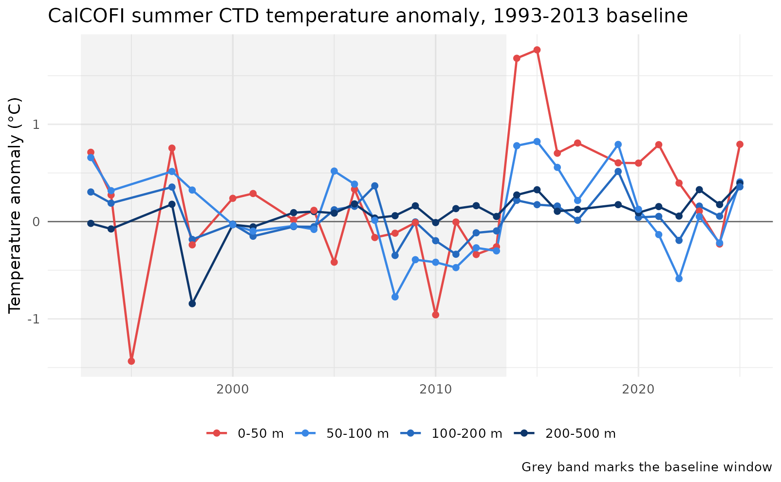

Summer temperature anomaly by year and depth layer

What the backfill is worth

The same analysis against a 1998–2013 baseline — what would have been possible before the 1993–2002 cruises were ingested.

clim_98 <- cc_climatology(
  con, variables = VAR, years = c(1998, 2013),
  depth_max = DEPTH_MAX, min_n = MIN_N) |>
  filter(clim_mean >= TEMP_RANGE_REGIONAL[1],
         clim_mean <= TEMP_RANGE_REGIONAL[2])

cmp <- obs_summer |>
  inner_join(clim_98, by = c("grid_key", "mon" = "month", "depth_m", "variable")) |>
  mutate(anomaly_98 = value - clim_mean) |>
  filter(depth_m <= 50) |>
  summarize(anomaly_98 = mean(anomaly_98), .by = yr)

comparison <- series |>
  filter(layer == "0-50 m") |>
  select(yr, anomaly_9313 = anomaly) |>
  inner_join(cmp, by = "yr") |>
  mutate(difference = anomaly_9313 - anomaly_98)

summary(abs(comparison$difference))
#>    Min. 1st Qu.  Median    Mean 3rd Qu.    Max. 
#> 0.04216 0.05814 0.06273 0.14239 0.24732 0.46284

Reading it honestly

The baseline is 21 years, not a 30-year WMO normal. CalCOFI’s 1 m-binned CTD record does not reach back far enough for one without splicing in ship hydrocast data of a different vintage. 1993–2013 does span both the 1997–98 El Niño and the 1998–99 La Niña, and it ends before the 2014–16 marine heatwave — so the heatwave and everything since read as departures rather than being folded into the normal.

Coverage is not constant. A spatial mean over “the line” covers different ocean in different years. The per-station differencing above removes each station’s own climate, which is most of the problem — but a year that skipped the offshore stations still has no offshore signal in it.

Preliminary cruises are fine for temperature, and not for the corrected series. Temperature is not bottle-corrected, so a preliminary_without_bottle cruise carries the temperature it always will. Salinity, oxygen and chlorophyll on those cruises are a different matter: the corrected forms do not exist until the bottle merge runs, and the uncorrected sensor series (salinity_1, oxygen_ml_l_1) are what is available.

The two-sensor averages are recomputed during ingest, not taken as shipped. The source CSVs carry pre-computed TempAve, SaltAve_Corr, OxAve_StaCorr and OxAveuM_StaCorr, and where one sensor is missing or has failed those sometimes fold the bad sensor in. The obvious form averages in the -99 missing marker; the dangerous form does not — a failed sensor reading −18 °C beside a good one at 20 °C yields an average of 0.77 °C, which is inside any plausible range and worth an 18 °C false cold anomaly. The ingest treats a sensor outside its declared bounds as absent and averages over what remains. Reading the source CSVs directly gives you the unrepaired values; see Q21.