---
title: "The CalCOFI grid from the official station positions"
subtitle: "One cell per official station: the rebuilt grid, its six acceptance gates and a variant, measured on v2026.10.01"
author: "CalCOFI"
date: today
format:
html:
toc: true
toc-depth: 3
code-fold: true
code-tools: true
fig-align: center
editor_options:
chunk_output_type: console
---
## Why, and where this stands {#sec-why}
Ben, 2026-10-02 ([CalCOFI/workflows#130](https://github.com/CalCOFI/workflows/issues/130)):
a grid point, i.e. a **site** (x: station, y: line), must land on its line, and the grid has
**slivers** (the [calcofi4r "CalCOFI grid"
figure](https://calcofi.io/calcofi4r/articles/calcofi4r.html#calcofi-grid); related
[#86](https://github.com/CalCOFI/workflows/issues/86) and
[CalCOFI/db-viz-station#19](https://github.com/CalCOFI/db-viz-station/issues/19)). Rather than
patch, start from the [official station
positions](https://calcofi.org/sampling-info/station-positions/) and build the cells as a Voronoi
tessellation of them.
The first version of this page (2026-10-02) compared that idea (Option A) with two repairs of the
previous grid. **On 2026-10-04 Ben decided that Option A ships in the next database release**,
and, the same day, that "kept from the previous grid" is literal: the previous cells beyond the
official pattern keep their own boundaries, and the station cells are confined to the previous
cells they replace (@sec-option-a).
The cells are now built by `calcofi4r::cc_grid_build()` and bundled as `calcofi4r::cc_grid`;
`calcofi4db::assign_grid_key()` keys a position to a cell, and the release publishes a
`grid_crosswalk` table. This page is the **evidence pack** for that implementation: the six
gates an independent review set (@sec-gates), each measured here on the promoted release
v2026.10.01, and the same headline numbers for one variant (no SCCOOS inshore cells) to put
beside it at the 2026-10-08 meeting.
This is an **exploration**, not an ingest. It has no `calcofi:` block, like every other
`explore_*.qmd`, so `build_targets_list()` never sees it: it is not a target, not a release
input, and it writes nothing to `cc_stage_dir()`. It changes no `grid_key`. It reads the published
release v2026.10.01 (the local copy under `cc_stage_dir()/releases/` when there is one) and writes
only this page.
::: {.callout-tip title="Short answer"}
The gate table is @tbl-gates; the shipped grid beside the variant and the two repairs is
@tbl-headline.
:::
```{r}
#| label: setup
librarian::shelf(DBI, dplyr, tidyr, ggplot2, glue, purrr, readr, sf, DT, quiet = T)
# the packages under review. A render before they are installed (a worktree) names their checkouts
# in CALCOFI4R_DIR / CALCOFI4DB_DIR and loads those; otherwise the installed packages are used
for (p in c("calcofi4r", "calcofi4db")) {
  d <- Sys.getenv(paste0(toupper(p), "_DIR"))
  if (nzchar(d)) suppressMessages(devtools::load_all(d, quiet = TRUE)) else library(p, character.only = TRUE)
}
stopifnot("this page needs the calcofi4r that carries the rebuilt grid (cc_grid_v1, cc_grid_build())" =
            exists("cc_grid_v1") && exists("cc_grid_build"),
          "this page needs the calcofi4db that builds the crosswalk (build_grid_crosswalk())" =
            exists("build_grid_crosswalk"))
options(dplyr.summarise.inform = FALSE)
suppressMessages(sf_use_s2(FALSE))  # planar on lon/lat, the predicate DuckDB's ST_Intersects uses in assign_grid_key()

ver      <- "v2026.10.01"       # the promoted release on 2026-10-02
CRS_M    <- 3310                # NAD83 / California Albers (m): every area, length and Voronoi below
KM_LINE  <- 22.2124             # km per line unit    (+proj=calcofi, measured below)
KM_STA   <- 7.3864              # km per station unit (+proj=calcofi, 4 nmi)
OFF_KM   <- 1                   # a site more than this from its line is "off its line"
SLIVER_W <- 2                   # km: a part narrower than this (mean width 2A/P) is a sliver ...
NOM_5    <- 5 * KM_STA * (10/3) * KM_LINE   # nominal area of a 5-unit nearshore cell, km²
SLIVER_A <- 0.25 * NOM_5        # km²: ... or smaller than a quarter of a 5-unit cell
CLIM_YR  <- c(1993, 2013)       # climatology window (build_climatology() default)
ERA_YR   <- 1984                # the 75-station pattern is standard from 1984

source(here::here("libs/reference_layers.R"))   # read_osm_land(): the release's land mask

# helpers ----
# polygon parts of a keyed sf, with area (km²) and mean width 2A/P (km)
split_parts <- function(x, key = "grid_key") {
  p <- x |> select(all_of(key)) |> st_cast("MULTIPOLYGON") |> st_cast("POLYGON", warn = FALSE)
  p$area_km2 <- as.numeric(st_area(p)) / 1e6
  p$width_km <- 2 * p$area_km2 / (as.numeric(st_length(st_cast(st_geometry(p), "MULTILINESTRING"))) / 1000)
  p |> group_by(across(all_of(key))) |>
    mutate(part = row_number(), n_parts = n(), largest = area_km2 == max(area_km2)) |> ungroup()
}
# a part is a sliver when it does not hold its cell's generator (the station it is the cell of)
# and it is thin or small
flag_slivers <- function(parts, gen, key = "grid_key") {
  hit <- mapply(function(p, k) {
    gi <- which(gen[[key]] == k); length(gi) && st_intersects(p, st_geometry(gen)[gi], sparse = FALSE)[1, 1]
  }, st_geometry(parts), parts[[key]])
  parts$holds_gen <- hit
  parts$sliver    <- !hit & (parts$width_km < SLIVER_W | parts$area_km2 < SLIVER_A)
  # a sliver touching another cell is the visible defect; one touching none is a pocket of
  # water the land mask cuts off (a lagoon, a harbour)
  nb <- st_is_within_distance(parts, parts, 50)
  parts$touches_other <- mapply(function(i, k) any(parts[[key]][i] != k), nb, parts[[key]])
  parts
}
# absorb every sliver into the neighbouring cell it shares the longest edge with,
# smallest first; a sliver with no neighbour keeps its key (reported)
absorb_slivers <- function(parts, key = "grid_key", tol_m = 50) {
  parts$key_new  <- parts[[key]]
  parts$shared_m <- NA_real_
  for (pid in order(parts$area_km2)) {
    if (!parts$sliver[pid]) next
    me     <- parts[pid, ]
    others <- which(parts$key_new != me$key_new)
    cand   <- others[st_intersects(st_buffer(st_geometry(me), tol_m), st_geometry(parts)[others], sparse = FALSE)[1, ]]
    if (!length(cand)) next
    bnd <- st_boundary(st_geometry(me))
    len <- vapply(cand, function(j) {
      x <- st_intersection(bnd, st_buffer(st_geometry(parts)[j], tol_m))
      if (!length(x) || all(st_is_empty(x))) 0 else sum(as.numeric(st_length(x)))
    }, numeric(1))
    if (max(len) <= 0) next
    parts$key_new[pid]  <- parts$key_new[cand[which.max(len)]]
    parts$shared_m[pid] <- max(len)
  }
  parts
}
# the cell a point falls in, in metres (the key that sorts first on a tie, as cc_grid_key())
first_hit <- function(pts, cells, key = "grid_key") {
  ix <- st_intersects(pts, cells)
  vapply(ix, function(i) if (length(i)) sort(cells[[key]][i], method = "radix")[1] else NA_character_, "")
}
# a site's distance from its line, km (+proj=calcofi via calcofi4db, never re-implemented)
off_line_km <- function(lon, lat, line) {
  p <- cc_lonlat_to_calcofi(lon, lat)
  abs(p$line - line) * KM_LINE
}
n_vertices <- function(x) sum(vapply(st_geometry(x), function(g) nrow(st_coordinates(g)), 1))
fmt <- function(x, d = 0) format(round(x, d), big.mark = ",", nsmall = d, trim = TRUE)
pct <- function(x, d = 1) paste0(format(round(100 * x, d), nsmall = d, trim = TRUE), "%")
```
## How the previous grid was built {#sec-today-build}
The release's `grid` table through v2026.10.01 (218 cells) is `calcofi4r::cc_grid` as it was
through calcofi4r 1.24.2, kept now as `calcofi4r::cc_grid_v1`, with each cell named
`st{station}-ln{line}` (`_hist` for the historical pattern). Every ingest calls
`calcofi4db::assign_grid_key()`, a point-in-polygon test of the sample's position against those
cells, so `grid_key` on `sample` and `obs` is wherever the position falls.
That grid came from `calcofi4r/data-raw/cc_grid_v1.R`, which:
1. lays three **idealized lattices** in `+proj=calcofi` (line, station) coordinates, not the
occupied positions: 5-unit spacing for stations ≤ 60 on the standard lines, 10-unit spacing
offshore to station 120, and a 20-unit historical lattice out to the convex hull of every
CTD cast;
2. takes a Voronoi tessellation of each lattice (in line/station units), cuts the finer ones
out of the coarser, and hand-merges six historical pairs (e.g. 55/80 from 50/80 + 60/80);
3. keeps the cells listed in `data-raw/cc_grid_sta-keys.csv` and erases Natural Earth 10 m land
(`st_difference`), which leaves gaps along the coast;
4. glues five of those gaps back onto line 93.3 cells by hand (`cc_grid_box4slivers.geojson`,
`st_union` onto `93.3,30` … `93.3,110`), which is where the line-93.3 cells pick up second,
detached parts;
5. makes the site of each cell `st_centroid(geom, of_largest_polygon = TRUE)` on lon/lat
(`cc_grid_ctrs`; the release's `grid.geom_ctr`).
So a site was the centroid of whatever polygon survived steps 2–4, never a station position:
that is why sites left their line wherever land, a merge or a glued gap reshaped the cell. And
the lattice is nominal (35, 40, 45, 50 …) while the occupied stations are not (90.0 37, 90.0 53,
80.0 51, 83.3 39.4 …), which is why an inshore cell held several real stations.
```{r}
#| label: read-release
cat_ <- NULL                    # the release catalog, fetched only when there is no local copy
con  <- get_duckdb_con(":memory:")
invisible(dbExecute(con, "SET memory_limit = '3GB'")); invisible(dbExecute(con, "SET threads = 2"))
invisible(dbExecute(con, "INSTALL httpfs; LOAD httpfs; INSTALL spatial; LOAD spatial"))
# the local copy of the release when this machine has one (release_database.qmd's stage dir), else https
dir_rel <- path.expand(file.path("~/_big/calcofi/releases", ver, "parquet"))
rp <- function(tbl) {
  f <- file.path(dir_rel, paste0(tbl, ".parquet")); d <- file.path(dir_rel, tbl)
  if (file.exists(f)) glue("read_parquet('{f}')")
  else if (dir.exists(d)) glue("read_parquet('{d}/**/*.parquet', hive_partitioning = true)")
  else {
    if (is.null(cat_)) cat_ <<- cc_catalog(ver)
    cc_read_parquet_sql(cc_release_sources(cat_, tbl))
  }
}

gr <- dbGetQuery(con, glue("
  SELECT grid_key, line, station, shore, pattern, spacing, area_km2,
         ST_AsWKB(geom) AS wkb, ST_AsWKB(geom_ctr) AS wkb_ctr
  FROM {rp('grid')}"))
grid <- st_sf(
  select(gr, -wkb, -wkb_ctr),
  geom = st_as_sfc(structure(gr$wkb, class = "WKB"), crs = 4326))
grid_ctr <- st_as_sfc(structure(gr$wkb_ctr, class = "WKB"), crs = 4326)

# the release grid is calcofi4r::cc_grid_v1, cell for cell
stopifnot(setequal(cc_grid_v1$grid_key, grid$grid_key))
n_same_geom <- sum(mapply(function(a, b) isTRUE(all.equal(a, b)),
                          st_geometry(grid), st_geometry(cc_grid_v1)[match(grid$grid_key, cc_grid_v1$grid_key)]))

# sample: one local copy (26 MB)
invisible(dbExecute(con, glue("
  CREATE TABLE sample AS
  SELECT sample_key, sample_type, parent_sample_key, dataset_key, grid_key, site_key, cruise_key,
         datetime, longitude, latitude
  FROM {rp('sample')}")))
invisible(dbExecute(con, glue(
  "CREATE TABLE climatology AS SELECT dataset_key, site_key, grid_key, month FROM {rp('climatology')}")))
n_sample <- dbGetQuery(con, "SELECT count(*) n FROM sample")$n
cat(glue("{ver} ({if (dir.exists(dir_rel)) 'local copy' else 'https'}): grid {nrow(grid)} cells ",
         "({n_same_geom} identical to calcofi4r::cc_grid_v1); sample {fmt(n_sample)} rows; climatology datasets ",
         "{paste(dbGetQuery(con, 'SELECT DISTINCT dataset_key FROM climatology ORDER BY 1')$dataset_key, collapse = ', ')}"), "\n")
```
## The official station positions {#sec-official}
`libs/download_station_positions.R` fetches the page and its linked files and stops if the
page's table, the linked `CalCOFIStationOrder.csv` and `CalCOFI_113StationMap.kml` disagree; its
tidy output (fetched 2026-10-02) is bundled as `calcofi4r::cc_station_positions`, which is what
the grid is built from. It is checked here against the copy of the linked CSV this repo tracks
(`data/station-positions/CalCOFIStationOrder.csv`).
```{r}
#| label: official
st <- cc_station_positions
n_ros <- sum(st$sta_type == "ROS"); n_sccoos <- sum(st$sta_type == "SCCOOS")
csv <- read_csv(here::here("data/station-positions/CalCOFIStationOrder.csv"), show_col_types = FALSE)
names(csv) <- sub("^", "", names(csv))
stopifnot(
  "the bundled station table is not the tracked CalCOFIStationOrder.csv" =
    nrow(csv) == nrow(st) &&
    isTRUE(all.equal(as.numeric(csv$LINE), st$line)) && isTRUE(all.equal(as.numeric(csv$STA), st$station)) &&
    max(abs(as.numeric(csv$`LAT (DEC)`) - st$latitude)) < 1e-6 &&
    max(abs(as.numeric(csv$`LON (DEC)`) - st$longitude)) < 1e-6)
cat(glue("cc_station_positions: {nrow(st)} stations ({n_ros} ROS, {n_sccoos} SCCOOS) on {n_distinct(st$line)} lines; ",
         "{sum(st$in_75)} in the 75-station pattern; {sum(!is.na(st$navy_ops_area))} Navy rows; ",
         "identical to the tracked CalCOFIStationOrder.csv"), "\n")
```
What the page lists:
- **Station Position (Lat/Lon), Depth, and Type**: `r nrow(st)` stations, `r n_ros` typed ROS
and `r n_sccoos` SCCOOS, on `r n_distinct(st$line)` lines (60 to 93.4), with order occupied
and estimated depth. This is the **113-station pattern**.
- The **75-station pattern** (standard since 1984; summer and fall): "66 stations from San Diego
to Avila Beach" on the 6 lines 93.3 to 76.7, plus "9 additional coastal ~20 m SCCOOS stations".
In the table that is every row with line ≥ 76.7: `r sum(st$in_75)` rows.
- The **104-station pattern** (winter and spring) adds 29 stations on lines 73.3 to 60.0; the 113
pattern adds 9 more by sampling every 20 nm on line 66.7. The page does not say which 9, so
the 104 subset is not marked.
- **Navy Stations**: `r sum(!is.na(st$navy_ops_area))` standard-pattern stations Navy operations
may close, with the operations area.
- Not listed: any historical station (e.g. 90.0 32, occupied 1959–84), any line north of 60 or
south of 93.4, or the Baja and Gulf of California lines.
### Each position against `+proj=calcofi`
`calcofi4db::cc_lonlat_to_calcofi()` projects each official lon/lat to continuous (line,
station); the residual is that minus the station's label, and the distance is from the official
position to `cc_calcofi_to_lonlat()` of the label.
```{r}
#| label: tbl-residuals
#| tbl-cap: "Official positions against `+proj=calcofi`: residuals in line and station units and the distance (m) between the listed position and the projected label, by station type."
pr <- cc_lonlat_to_calcofi(st$longitude, st$latitude)
nm <- cc_calcofi_to_lonlat(st$line, st$station)
st <- st |> mutate(
  d_line = pr$line - line, d_sta = pr$station - station,
  dist_m = as.numeric(st_distance(
    st_as_sf(st, coords = c("longitude", "latitude"), crs = 4326),
    st_as_sf(nm, coords = c("longitude", "latitude"), crs = 4326), by_element = TRUE)))
# km per unit, measured (the constants in setup)
u <- cc_calcofi_to_lonlat(c(90, 91, 90), c(60, 60, 61))
suppressMessages(sf_use_s2(TRUE))
km_unit <- as.numeric(st_distance(st_as_sf(u, coords = c("longitude", "latitude"), crs = 4326))[1, 2:3]) / 1000
suppressMessages(sf_use_s2(FALSE))
stopifnot(abs(km_unit[1] - KM_LINE) < 0.01, abs(km_unit[2] - KM_STA) < 0.01)
st |> group_by(sta_type) |>
  summarize(
    n = n(),
    `max |Δ line|` = signif(max(abs(d_line)), 2), `max |Δ station|` = signif(max(abs(d_sta)), 2),
    `median distance (m)` = round(median(dist_m), 1), `max distance (m)` = round(max(dist_m), 1)) |>
  knitr::kable()
```
Every official position is its label under `+proj=calcofi` to within
**`r round(max(st$dist_m))` m** (`r signif(max(abs(st$d_sta)), 2)` station units at most): the
table is the projection, rounded. One line unit is `r round(km_unit[1], 2)` km and one station
unit `r round(km_unit[2], 3)` km (4 nmi). So an official position *is* on its line, and a
Voronoi built from them inherits that.
## The previous grid's defects {#sec-today}
```{r}
#| label: today
gm <- st_transform(grid, CRS_M)
nom_ll <- cc_calcofi_to_lonlat(grid$line, grid$station)
nom <- st_as_sf(cbind(st_drop_geometry(grid)[c("grid_key", "line", "station", "pattern")], nom_ll),
                coords = c("longitude", "latitude"), crs = 4326)
ctr_xy <- st_coordinates(grid_ctr)
ctr_c  <- cc_lonlat_to_calcofi(ctr_xy[, 1], ctr_xy[, 2])
grid <- grid |> mutate(
  ctr_line = ctr_c$line, ctr_sta = ctr_c$station,
  off_km   = abs(ctr_line - line) * KM_LINE,
  along_km = (ctr_sta - station) * KM_STA,
  nom_in_cell = mapply(function(p, c) st_intersects(p, c, sparse = FALSE)[1, 1],
                       st_geometry(nom), st_geometry(grid)))

# the coastline the release masks land with (OSM, ingest_spatial.qmd's reference layer), in full
# detail: the figures' land, and the measure of the gaps the previous grid left
bb   <- st_bbox(grid)
land_zip <- c(cc_stage_path("reference", OSM_LAND_ZIP),
              path.expand(file.path("~/_big/calcofi/reference", OSM_LAND_ZIP)))
land_zip <- land_zip[file.exists(land_zip)][1]
stopifnot("no OSM land-polygons zip: run ingest_spatial.qmd's reference layers first" = !is.na(land_zip))
land <- read_osm_land(
  land_zip,
  bbox = c(xmin = bb[["xmin"]] - .5, ymin = bb[["ymin"]] - .5, xmax = bb[["xmax"]] + .5, ymax = bb[["ymax"]] + .5))
land_m <- st_union(st_transform(st_make_valid(land), CRS_M))
# a light copy for the full-extent figures
land_lite <- st_transform(st_simplify(land_m, preserveTopology = TRUE, dTolerance = 1000), 4326)
LAND_FILL <- "#d8ccb4"          # land, in the figures whose cells are grey

# outer hull of the previous grid: the union with interior holes filled
hull_m  <- st_union(st_make_valid(gm))
outer_m <- st_union(st_sfc(
  lapply(st_geometry(st_cast(hull_m, "POLYGON")), function(p) st_polygon(list(p[[1]]))), crs = CRS_M))
gaps <- st_difference(st_difference(outer_m, hull_m), land_m) |> st_cast("POLYGON") |> st_sf()
gaps$area_km2 <- as.numeric(st_area(gaps)) / 1e6
gaps$at_coast <- st_is_within_distance(gaps, land_m, 100, sparse = FALSE)[, 1]

# slivers
parts_now <- split_parts(gm) |> left_join(st_drop_geometry(grid)[c("grid_key", "spacing", "pattern")], by = "grid_key")
parts_now <- flag_slivers(parts_now, st_transform(nom, CRS_M))

# official stations per cell
stp <- st_transform(st_as_sf(st, coords = c("longitude", "latitude"), crs = 4326, remove = FALSE), CRS_M)
stp$grid_key_now <- cc_grid_key(st$longitude, st$latitude, cc_grid_v1)
n_per_cell <- table(stp$grid_key_now)
```
```{r}
#| label: tbl-today
#| tbl-cap: "The previous grid (v2026.10.01 `grid`, 218 cells): sites off their line, slivers, gaps and cells holding several official stations."
today <- tribble(
  ~measure, ~value,
  "cells", fmt(nrow(grid)),
  glue("sites (geom_ctr) more than {OFF_KM} km off their line"), glue("{sum(grid$off_km > OFF_KM)} ({sum(grid$off_km > OFF_KM & grid$pattern != 'historical')} outside the historical pattern)"),
  "sites more than 0.1 km off their line", fmt(sum(grid$off_km > 0.1)),
  "largest distance of a site from its line (km)", fmt(max(grid$off_km), 1),
  "median distance of a site from its line (km)", fmt(median(grid$off_km), 2),
  "cells whose own station (label) lies outside the cell", fmt(sum(!grid$nom_in_cell)),
  "cells in more than one piece", fmt(sum(parts_now$part == 1 & parts_now$n_parts > 1)),
  glue("sliver parts (no station of their own; mean width < {SLIVER_W} km or area < {fmt(SLIVER_A)} km²)"),
    glue("{sum(parts_now$sliver)} of {nrow(parts_now)} parts ({sum(parts_now$sliver & parts_now$n_parts == 1)} whole cells, {sum(parts_now$sliver & parts_now$n_parts > 1)} pieces of multi-part cells; {sum(parts_now$sliver & parts_now$touches_other)} touch another cell)"),
  glue("  of which thinner than {SLIVER_W} km"), fmt(sum(parts_now$sliver & parts_now$width_km < SLIVER_W)),
  "gaps inside the outer hull that are neither a cell nor OSM land (> 1 km²)",
    glue("{sum(gaps$area_km2 > 1)} ({sum(gaps$area_km2 > 1 & !gaps$at_coast)} away from the coast), {fmt(sum(gaps$area_km2))} km² in all"),
  "cells holding ≥ 2 official stations", glue("{sum(n_per_cell >= 2)} (holding {sum(n_per_cell[n_per_cell >= 2])} of {nrow(st)} stations)"),
  "official stations outside every cell", fmt(sum(is.na(stp$grid_key_now))))
knitr::kable(today, col.names = c("", ""))
```
The sub-kilometre offsets are built into the lattice: the lines are 3.3 and 3.4 units apart in
turn (80, 83.3, 86.7, 90 …), and a Voronoi edge sits at the midpoint, so the centre of every cell
on lines 76.7, 83.3, 86.7 and 93.3 is 0.025 line units (about 0.55 km) off its line, while lines
80 and 90 sit almost on it (the median offset of a site on a 10-unit cell is
`r fmt(median(grid$off_km[grid$spacing == 10 & grid$line %in% c(76.7, 83.3, 86.7, 93.3)]), 2)` km
on those four lines and
`r fmt(median(grid$off_km[grid$spacing == 10 & grid$line %in% c(80, 90)]), 2)` km on 80 and 90).
The large offsets are the cells that land, a hand-merge or a glued gap reshaped (@tbl-offline).
```{r}
#| label: tbl-offline
#| tbl-cap: "Sites of the previous grid more than 1 km off their line, outside the historical pattern: the site's continuous (line, station) under `+proj=calcofi`, its distance across the line and along it, the cell's area and whether its own station label is inside the cell."
grid |> st_drop_geometry() |>
  filter(off_km > OFF_KM, pattern != "historical") |>
  arrange(desc(off_km)) |>
  transmute(grid_key, pattern, area_km2 = round(area_km2),
            site = sprintf("%.2f / %.2f", ctr_line, ctr_sta),
            `off line (km)` = round(off_km, 1), `along line (km)` = round(along_km, 1),
            `station in cell` = nom_in_cell) |>
  knitr::kable()
```
```{r}
#| label: tbl-multi
#| tbl-cap: "Cells of the previous grid that hold two or more official stations (113-station table)."
stp |> st_drop_geometry() |> filter(!is.na(grid_key_now)) |>
  group_by(grid_key = grid_key_now) |>
  summarize(n = n(), stations = paste(sprintf("%.1f %.1f%s", line, station, ifelse(sta_type == "SCCOOS", " (SCCOOS)", "")), collapse = "; ")) |>
  filter(n >= 2) |> arrange(desc(n), grid_key) |> knitr::kable()
```
```{r}
#| label: fig-today
#| warning: false
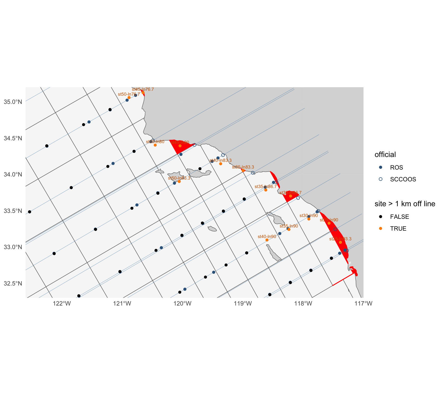
#| fig-cap: "The previous grid in the Southern California Bight and Point Conception: cells (grey; slivers red), sites (`grid.geom_ctr`; orange where more than 1 km off their line), official stations (blue; SCCOOS hollow) and the CalCOFI lines (thin)."
#| fig-height: 8
#| fig-width: 9
lines_ll <- map_dfr(sort(unique(st$line)), function(l) {
  s <- seq(20, 125, by = 0.5); ll <- cc_calcofi_to_lonlat(l, s); tibble(line = l, lon = ll$longitude, lat = ll$latitude)
}) |> st_as_sf(coords = c("lon", "lat"), crs = 4326) |> group_by(line) |> summarize(do_union = FALSE) |> st_cast("LINESTRING")
zoom <- coord_sf(xlim = c(-122.6, -117), ylim = c(32.3, 35.2), expand = FALSE)
site_pts <- st_sf(grid_key = grid$grid_key, off = grid$off_km > OFF_KM, geom = grid_ctr)
ggplot() +
  geom_sf(data = land, fill = "grey85", color = NA) +
  geom_sf(data = grid, fill = "grey97", color = "grey45", linewidth = 0.3) +
  geom_sf(data = st_transform(filter(parts_now, sliver), 4326), fill = "red", color = "red", linewidth = 0.6) +
  geom_sf(data = lines_ll, color = "steelblue", linewidth = 0.2, alpha = 0.6) +
  geom_sf(data = stp |> st_transform(4326), aes(shape = sta_type), color = "steelblue4", size = 1.8) +
  geom_sf(data = site_pts, aes(color = off), size = 1.4) +
  geom_sf_text(data = filter(site_pts, off), aes(label = grid_key), size = 2.3, nudge_y = 0.05, color = "darkorange3") +
  scale_shape_manual(values = c(ROS = 16, SCCOOS = 1), name = "official") +
  scale_color_manual(values = c(`FALSE` = "black", `TRUE` = "darkorange"), name = "site > 1 km off line") +
  zoom + theme_minimal() + labs(x = NULL, y = NULL)
```
## The shipped grid: one cell per official station, inside the previous grid {#sec-option-a}
`calcofi4r::cc_grid` is `cc_grid_build(cc_station_positions, cc_grid_v1, cc_grid_land)`
(`calcofi4r/data-raw/cc_grid.R`, no hand edits). The rules, as the function documents them:
1. **Extent.** The outer hull of the previous grid (the union of its cells with interior holes
filled) minus land.
2. **Kept or replaced.** A previous cell whose labelled (line, station) lies more than 20
nautical miles outside the convex hull of the `r nrow(st)` official stations is **kept**; the
others are **replaced**. Where two previous cells overlap, the overlap is the cell whose key
sorts first, the cell a position there keyed to.
3. **Kept cells are the previous cells.** A kept cell keeps its key, its attributes and its own
boundaries, toward the other kept cells and toward the replaced region, so a historical
position that was in a kept cell is still in it. Only its coast side changes: it ends at the
new land.
4. **Station cells.** The Voronoi tessellation of the official positions in metres (California
Albers, not line/station units, which weigh a line unit of 22.2 km and a station unit of 7.4 km
alike), **confined to the replaced region R** (the union of the replaced cells): an outer
station's cell stops where the previous lattice stopped it, at line 95.0 in the south (20
nautical miles beyond line 93.3). Each edge gets a vertex every 5 km so the lon/lat polygon
follows the metric edge.
5. **Pockets.** A piece of a station's cell that land separates from the piece holding the
station joins the neighbouring station cell it shares the longest water edge with. A pocket
never joins a kept cell. Water of R that no station cell reaches stays with the station it is
nearest to, as a detached part, and is reported (@tbl-cases).
6. **Gap water.** Water of the extent that no previous cell covered (the previous grid was
clipped by a coarser coastline) joins the cell whose edge it is nearest to, kept or replaced.
Gap water that touches no cell is left out.
7. **Sites.** A station cell's site (`grid.geom_ctr`) is the station. A kept cell's site is its
label under `+proj=calcofi` when the cell holds it, else the previous cell's centre, else a
point on the cell.
8. **Attributes.** A station's cell is `nearshore` at station ≤ 60 and `offshore` beyond;
`standard` on lines ≥ 76.7 (the 75-station pattern) and `extended` north of it; spacing class 5
nearshore, 10 offshore. A kept cell keeps the previous cell's attributes.
The land is `calcofi4r::cc_grid_land`: OpenStreetMap land polygons
(extract `r cc_grid_land$version`) with islets under 1 km² dropped, the coastline pulled back
300 m and simplified to 100 m, so a ship at its berth or a nearshore position rounded to the
minute still falls in a cell and the cells stay light enough for a browser.
**Why the station cells are confined.** A first build let the official Voronoi run to the
bisector with the kept cells' labels. The outer official cells then reached 40 nautical miles
beyond line 93.3 (halfway to the line-100 lattice), where the previous lattice gave them 20, and
historical line 96.7 fell on the new edge: 18,795 of its 28,367 `sample` rows left the line-100
cells and seven of its stations were split between two cells. Confining the station cells to R
puts every boundary of the previous grid that was not inside the official pattern back where it
was (@tbl-line967, @tbl-kept).
```{r}
#| label: option-a
# the shipped cells, and the same build re-run from the bundled inputs for what it reports
# (which previous cell became what, the pockets that changed cell, the water it dropped)
b_ship <- cc_grid_build()
stopifnot(
  "the bundled cc_grid is not cc_grid_build() of the bundled inputs" =
    identical(b_ship$grid$grid_key, cc_grid$grid_key) &&
    isTRUE(all.equal(as.numeric(st_area(st_transform(b_ship$grid, CRS_M))),
                     as.numeric(st_area(st_transform(cc_grid, CRS_M))), tolerance = 1e-9)))
A      <- st_transform(cc_grid, CRS_M) |> transmute(grid_key, line = sta_lin, station = sta_pos,
            gen_source = sta_source, sta_type, zone_key)
A$area_km2 <- as.numeric(st_area(A)) / 1e6
gen_a  <- st_transform(cc_grid_ctrs, CRS_M) |> transmute(grid_key, line = sta_lin, station = sta_pos,
            gen_source = sta_source, sta_type)
parts_a_after <- flag_slivers(split_parts(A), gen_a)
# the site of a cell is its generator: on its line by construction
A_site <- st_transform(gen_a, 4326)
A_off  <- off_line_km(st_coordinates(A_site)[, 1], st_coordinates(A_site)[, 2], A_site$line)
prevt  <- b_ship$prev
kept_keys <- prevt$grid_key[prevt$fate == "kept"]
n_parts   <- function(x) vapply(st_geometry(x), function(g) if (inherits(g, "MULTIPOLYGON")) length(g) else 1L, 1L)
rp_    <- as.list(b_ship$report)
cat(glue(
  "shipped: {rp_$cells} cells = {rp_$stations} station cells + {rp_$kept} kept from the previous grid ",
  "(site at the label {sum(prevt$site_at == 'label', na.rm = TRUE)}, at the previous centre {sum(prevt$site_at == 'centre', na.rm = TRUE)}, ",
  "on the cell {sum(prevt$site_at == 'water', na.rm = TRUE)}); {rp_$replaced} previous cells replaced; ",
  "{rp_$pockets_moved} pockets joined a neighbouring station cell; {rp_$multipart_cells} multi-part cells ",
  "({rp_$multipart_official} of them a station cell); gap water joined to kept cells {fmt(sum(prevt$gap_km2))} km²; ",
  "{rp_$dropped_water} gap waters left out ({fmt(sum(b_ship$dropped$area_km2), 1)} km²); {rp_$cases} case(s) reported; ",
  "{fmt(n_vertices(cc_grid))} vertices (previous grid {fmt(n_vertices(cc_grid_v1))})"), "\n")
```
```{r}
#| label: tbl-option-a-cells
#| tbl-cap: "The shipped grid: cells by source, station type and zone, with their area (km²)."
A |> st_drop_geometry() |>
  group_by(source = gen_source, `station type` = sta_type, zone = zone_key) |>
  summarize(n = n(), min = round(min(area_km2), 1), median = round(median(area_km2)), max = round(max(area_km2))) |>
  knitr::kable(format.args = list(big.mark = ","))
```
```{r}
#| label: fig-shipped-full
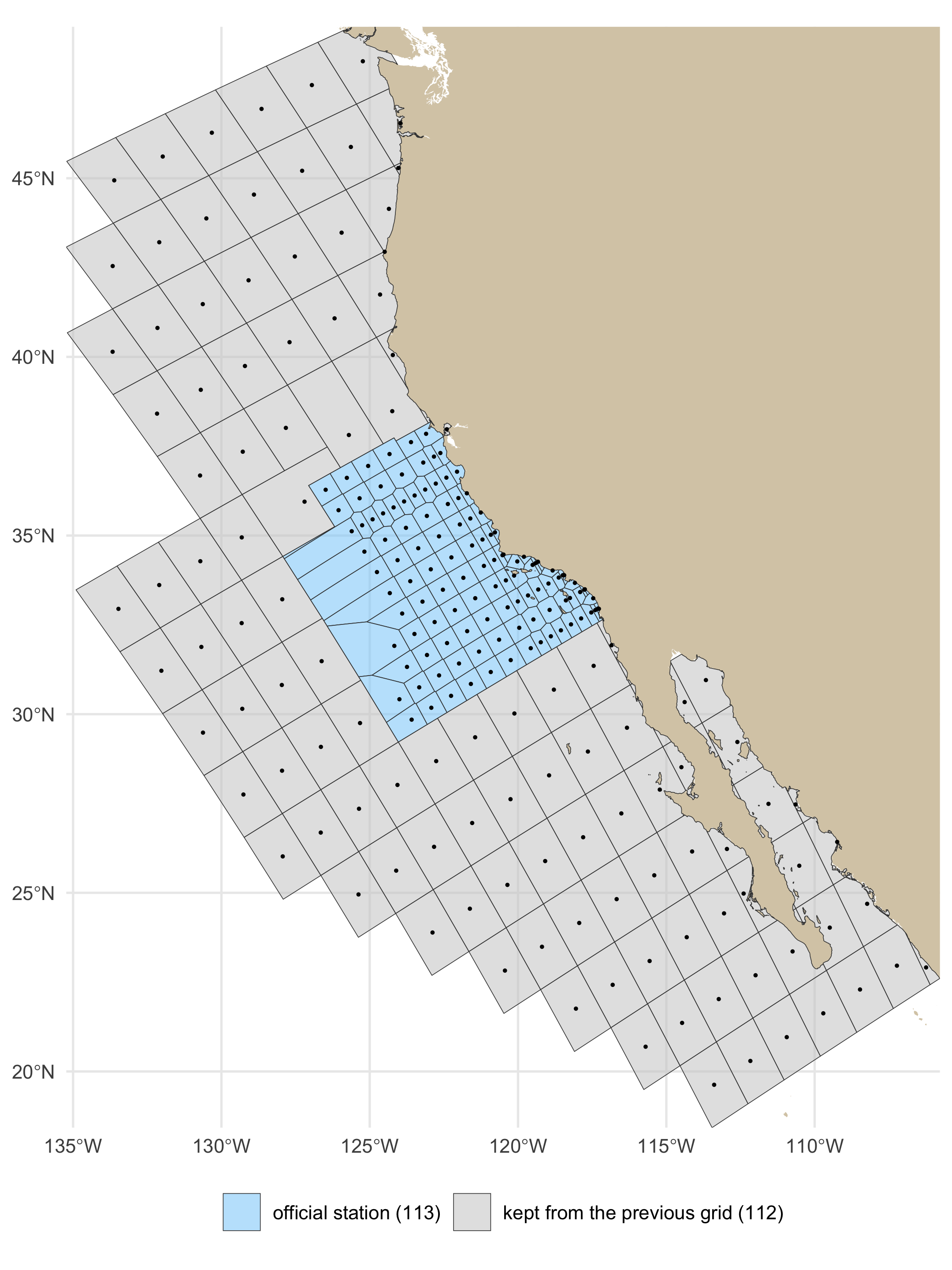
#| fig-cap: "The shipped grid over its full extent: cells of the official stations (blue) and the cells kept from the previous grid (grey), each with its site. The previous outer hull bounds it offshore; land is the OpenStreetMap coastline."
#| fig-height: 8
#| fig-width: 6
#| dpi: 180
ggplot() +
  geom_sf(data = land_lite, fill = LAND_FILL, color = NA) +
  geom_sf(data = cc_grid, aes(fill = sta_source), color = "grey25", linewidth = 0.15, alpha = 0.55) +
  geom_sf(data = cc_grid_ctrs, size = 0.25) +
  scale_fill_manual(values = c(official = "lightskyblue", previous = "grey80"),
                    labels = c(official = "official station (113)", previous = "kept from the previous grid (112)"), name = NULL) +
  coord_sf(xlim = c(bb[["xmin"]], bb[["xmax"]]), ylim = c(bb[["ymin"]], bb[["ymax"]]), expand = FALSE) +
  theme_minimal(base_size = 11) + theme(legend.position = "bottom") + labs(x = NULL, y = NULL)
```
```{r}
#| label: fig-shipped-pattern
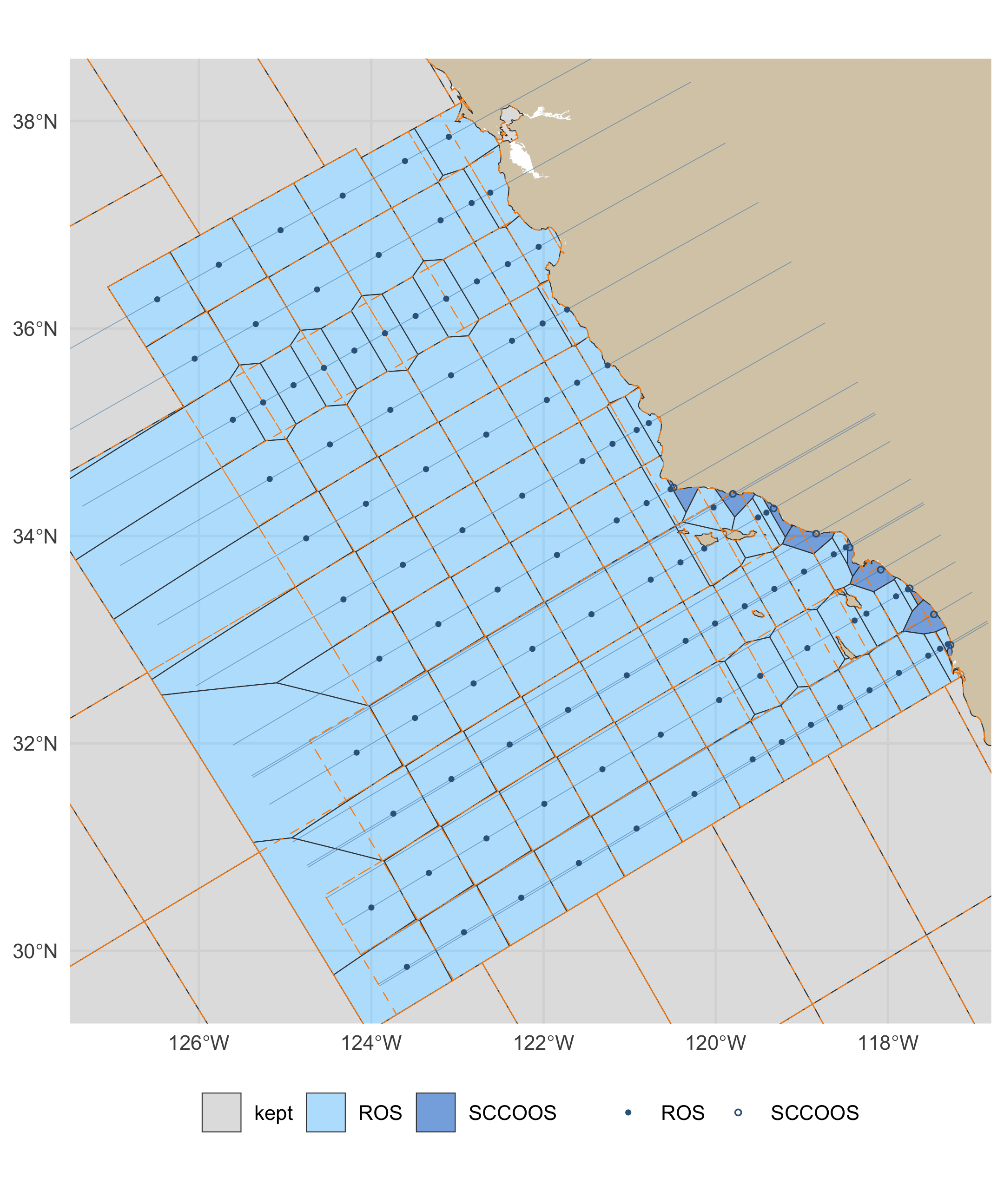
#| fig-cap: "The official pattern, lines 60 to 93.4 out to station 120: the shipped cells (blue official, SCCOOS darker; grey kept) with the previous grid's edges dashed in orange, the CalCOFI lines (thin) and the official stations (SCCOOS hollow)."
#| fig-height: 7.2
#| fig-width: 6
#| dpi: 180
cell_fill <- ifelse(cc_grid$sta_source == "previous", "kept", ifelse(cc_grid$sta_type == "SCCOOS", "SCCOOS", "ROS"))
ggplot() +
  geom_sf(data = land_lite, fill = LAND_FILL, color = NA) +
  geom_sf(data = mutate(cc_grid, f = cell_fill), aes(fill = f), color = "grey25", linewidth = 0.2, alpha = 0.6) +
  geom_sf(data = grid, fill = NA, color = "darkorange", linewidth = 0.2, linetype = "dashed") +
  geom_sf(data = lines_ll, color = "steelblue", linewidth = 0.15, alpha = 0.6) +
  geom_sf(data = filter(A_site, gen_source == "official"), aes(shape = sta_type), color = "steelblue4", size = 0.9) +
  scale_shape_manual(values = c(ROS = 16, SCCOOS = 1), name = NULL) +
  scale_fill_manual(values = c(ROS = "lightskyblue", SCCOOS = "dodgerblue3", kept = "grey80"), name = NULL) +
  coord_sf(xlim = c(-127.5, -116.8), ylim = c(29.3, 38.6), expand = FALSE) +
  theme_minimal(base_size = 11) + theme(legend.position = "bottom") + labs(x = NULL, y = NULL)
```
```{r}
#| label: fig-shipped-north
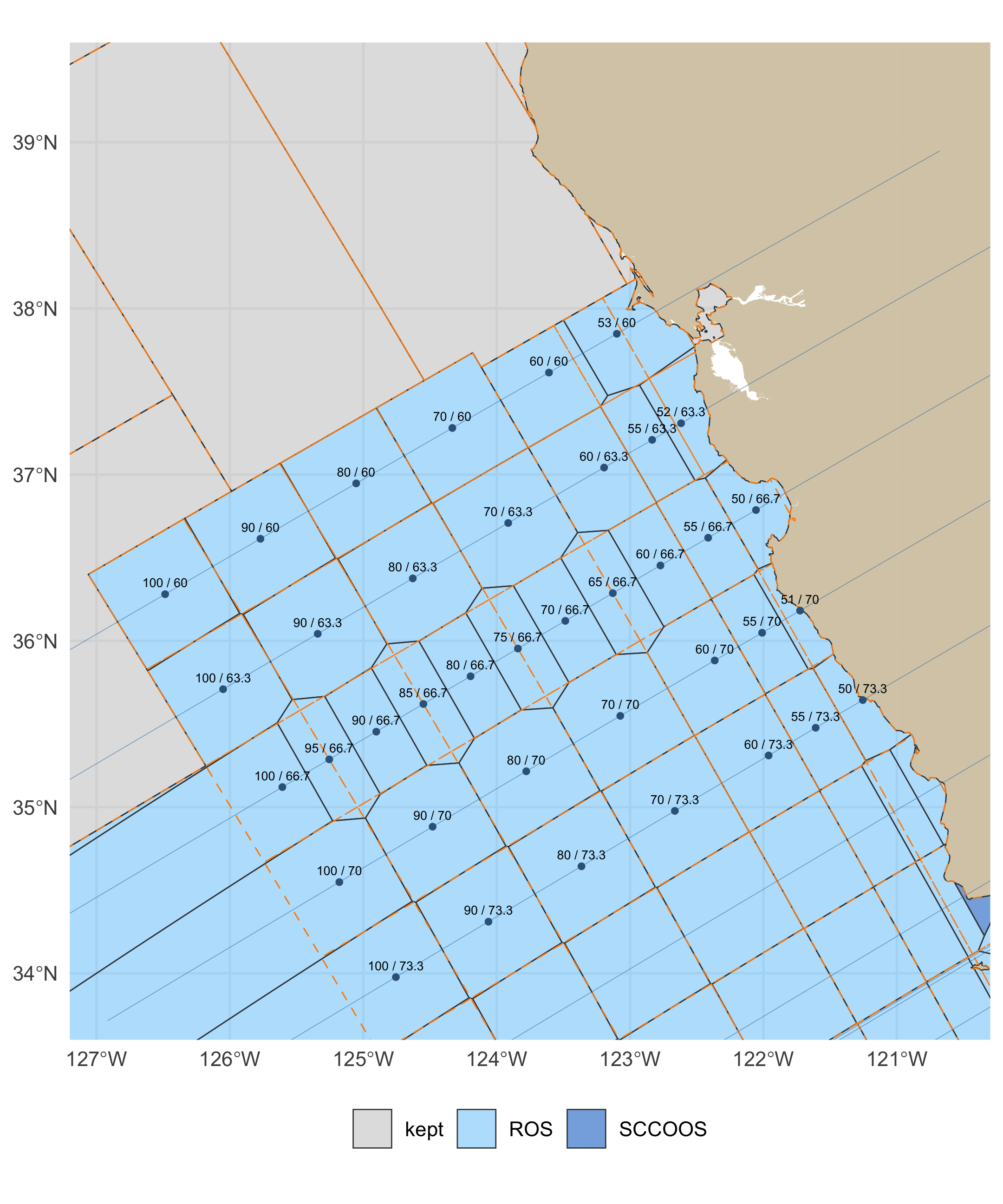
#| fig-cap: "Lines 60 to 73.3 (the extended pattern, San Francisco to Point Conception) and the kept cells north of them: shipped cells, the previous edges dashed in orange, and each official cell's station / line."
#| fig-height: 7.2
#| fig-width: 6
#| dpi: 180
lab_n <- filter(A_site, gen_source == "official", line < 76.7)
ggplot() +
  geom_sf(data = land, fill = LAND_FILL, color = NA) +
  geom_sf(data = mutate(cc_grid, f = cell_fill), aes(fill = f), color = "grey25", linewidth = 0.25, alpha = 0.6) +
  geom_sf(data = grid, fill = NA, color = "darkorange", linewidth = 0.25, linetype = "dashed") +
  geom_sf(data = lines_ll, color = "steelblue", linewidth = 0.15, alpha = 0.6) +
  geom_sf(data = lab_n, color = "steelblue4", size = 0.9) +
  geom_sf_text(data = lab_n, aes(label = sub("^st", "", sub("-ln", " / ", grid_key))), size = 1.9, nudge_y = 0.07) +
  scale_fill_manual(values = c(ROS = "lightskyblue", SCCOOS = "dodgerblue3", kept = "grey80"), name = NULL) +
  coord_sf(xlim = c(-127.2, -120.3), ylim = c(33.6, 39.6), expand = FALSE) +
  theme_minimal(base_size = 11) + theme(legend.position = "bottom") + labs(x = NULL, y = NULL)
```
```{r}
#| label: fig-option-a
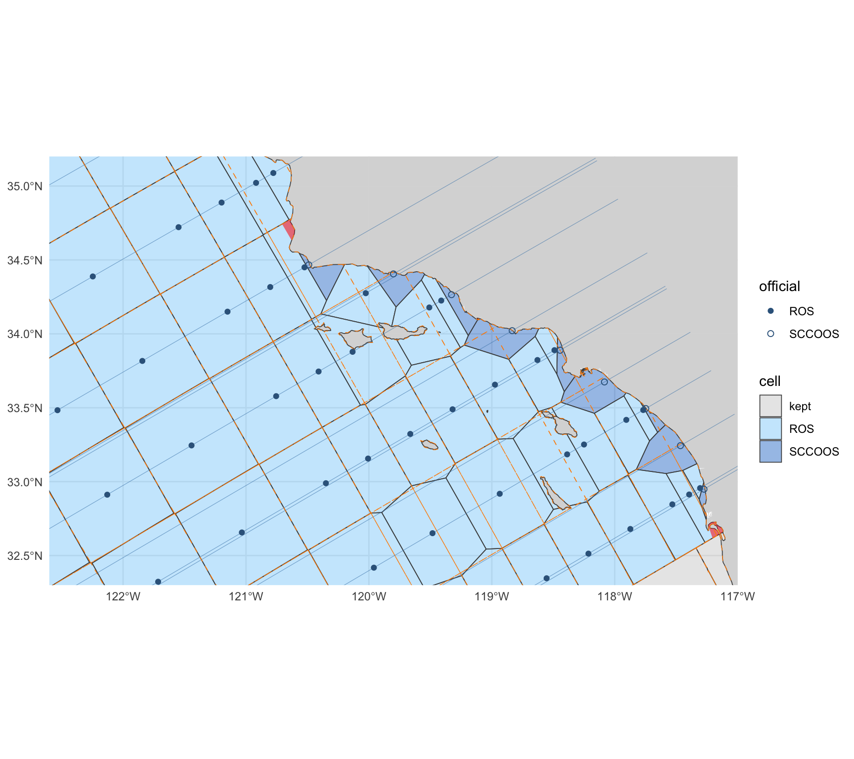
#| fig-cap: "The shipped grid in the Southern California Bight and Point Conception: cells of the official stations (blue; SCCOOS darker), the previous grid's edges dashed in orange, and in red the pockets that joined a neighbour because land cuts them off from their nearest station."
#| fig-height: 8
#| fig-width: 9
ggplot() +
  geom_sf(data = land, fill = "grey85", color = NA) +
  geom_sf(data = mutate(cc_grid, f = cell_fill), aes(fill = f), color = "grey30", linewidth = 0.3, alpha = 0.45) +
  geom_sf(data = b_ship$pockets, fill = "red", color = NA, alpha = 0.55) +
  geom_sf(data = grid, fill = NA, color = "darkorange", linewidth = 0.25, linetype = "dashed") +
  geom_sf(data = lines_ll, color = "steelblue", linewidth = 0.2, alpha = 0.6) +
  geom_sf(data = filter(A_site, gen_source == "official"), aes(shape = sta_type), color = "steelblue4", size = 1.8) +
  scale_shape_manual(values = c(ROS = 16, SCCOOS = 1), name = "official") +
  scale_fill_manual(values = c(ROS = "lightskyblue", SCCOOS = "dodgerblue3", kept = "grey80"), name = "cell") +
  zoom + theme_minimal() + labs(x = NULL, y = NULL)
```
## Two repairs of the previous grid, for comparison {#sec-repairs}
### Option B: keep the cells, absorb the slivers {#sec-option-b}
Every sliver part of the previous grid (the rule in @tbl-today) joins the neighbouring cell it
shares the longest edge with, smallest first. A whole-cell sliver retires its key. Sites are
recomputed as the previous build does (centroid of the largest polygon).
```{r}
#| label: option-b
parts_b <- absorb_slivers(parts_now)
B <- parts_b |> group_by(grid_key = key_new) |> summarize()
B_site <- suppressWarnings(st_centroid(st_transform(B, 4326), of_largest_polygon = TRUE)) |>
  left_join(st_drop_geometry(grid)[c("grid_key", "line", "pattern")], by = "grid_key")
B_off <- off_line_km(st_coordinates(B_site)[, 1], st_coordinates(B_site)[, 2], B_site$line)
retired_b <- setdiff(grid$grid_key, B$grid_key)
parts_b_after <- flag_slivers(split_parts(B), st_transform(nom, CRS_M))
cat(glue("B: {sum(parts_b$key_new != parts_b$grid_key)} of {sum(parts_b$sliver)} slivers absorbed; {nrow(B)} cells; ",
         "retired: {paste(retired_b, collapse = ', ')}"), "\n")
```
### Option C: keep the cells, move each site onto its line {#sec-option-c}
Each site moves to the nearest point of its line (in `+proj=calcofi`, the line is `x = line`)
that lies inside its own cell. Cells, and so every `grid_key`, are unchanged; only
`grid.geom_ctr` moves. A cell its own line does not cross cannot be fixed this way.
```{r}
#| label: option-c
gc <- st_transform(grid, st_crs("+proj=calcofi"))
c_sta <- vapply(seq_len(nrow(gc)), function(i) {
  ln  <- st_sfc(st_linestring(cbind(gc$line[i], c(-300, 400))), crs = st_crs(gc))
  seg <- st_intersection(ln, st_geometry(gc)[i])
  if (!length(seg) || all(st_is_empty(seg))) return(NA_real_)
  y <- vapply(st_geometry(st_cast(seg, "LINESTRING")), function(p) {
    r <- range(st_coordinates(p)[, "Y"]); min(max(grid$ctr_sta[i], r[1]), r[2]) }, numeric(1))
  y[which.min(abs(y - grid$ctr_sta[i]))]
}, numeric(1))
c_ll <- cc_calcofi_to_lonlat(grid$line, c_sta)
c_ok <- !is.na(c_sta)
suppressMessages(sf_use_s2(TRUE))
c_move_km <- rep(NA_real_, nrow(grid))
c_move_km[c_ok] <- as.numeric(st_distance(
  grid_ctr[c_ok], st_as_sfc(st_as_sf(c_ll[c_ok, ], coords = c("longitude", "latitude"), crs = 4326)), by_element = TRUE)) / 1000
suppressMessages(sf_use_s2(FALSE))
cat(glue("C: {sum(c_ok)} sites moved onto their line (median {round(median(c_move_km, na.rm = TRUE), 2)} km, ",
         "{sum(c_move_km > OFF_KM, na.rm = TRUE)} by more than {OFF_KM} km, max {round(max(c_move_km, na.rm = TRUE), 1)} km); ",
         "{sum(!c_ok)} cells their line does not cross: {paste(grid$grid_key[!c_ok], collapse = ', ')}"), "\n")
```
## The variant: no SCCOOS inshore cells {#sec-variant}
The one variant to show beside the shipped grid on 2026-10-08: the same build seeded from the
regular station pattern only, i.e. the `r n_ros` ROS stations, so each of the nine ~20 m SCCOOS
stations falls in the cell of the nearest ROS station instead of having a cell of its own.
Everything else (extent, land, kept cells, pockets, attributes) is identical. It is not shipped.
```{r}
#| label: variant
b_var <- cc_grid_build(stations = filter(cc_station_positions, sta_type != "SCCOOS"))
V     <- st_transform(b_var$grid, CRS_M); V$area_km2 <- as.numeric(st_area(V)) / 1e6
rv_   <- as.list(b_var$report)
stopifnot("the variant keeps other previous cells than the shipped grid" =
            setequal(b_var$prev$grid_key[b_var$prev$fate == "kept"], kept_keys))
cat(glue("variant: {rv_$cells} cells = {rv_$stations} station cells + {rv_$kept} kept (the same {rv_$kept}); ",
         "{rv_$pockets_moved} pockets joined a neighbouring station cell; {rv_$multipart_cells} multi-part cells ",
         "({rv_$multipart_official} a station cell); {rv_$cases} case(s) reported"), "\n")
```
```{r}
#| label: fig-variant
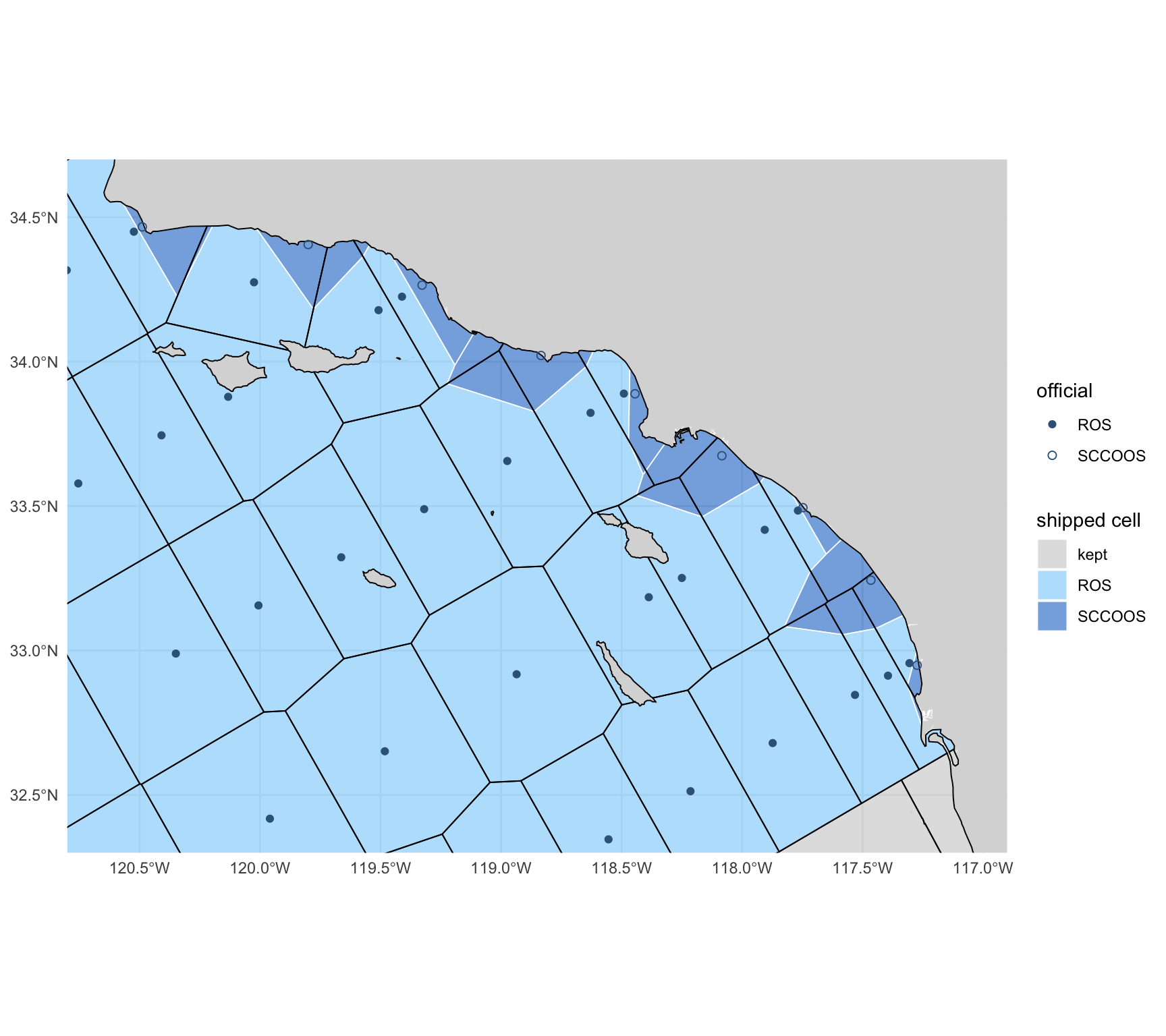
#| fig-cap: "The variant beside the shipped grid, inshore Southern California: shipped cells filled (SCCOOS cells darker), the variant's edges in black. Where there is no SCCOOS station the two coincide; each SCCOOS cell is absorbed by its ROS neighbours."
#| fig-height: 8
#| fig-width: 9
ggplot() +
  geom_sf(data = land, fill = "grey85", color = NA) +
  geom_sf(data = mutate(cc_grid, f = cell_fill), aes(fill = f), color = "white", linewidth = 0.3, alpha = 0.6) +
  geom_sf(data = b_var$grid, fill = NA, color = "black", linewidth = 0.35) +
  geom_sf(data = filter(A_site, gen_source == "official"), aes(shape = sta_type), color = "steelblue4", size = 1.8) +
  scale_shape_manual(values = c(ROS = 16, SCCOOS = 1), name = "official") +
  scale_fill_manual(values = c(ROS = "lightskyblue", SCCOOS = "dodgerblue3", kept = "grey80"), name = "shipped cell") +
  coord_sf(xlim = c(-120.8, -116.9), ylim = c(32.3, 34.7), expand = FALSE) + theme_minimal() + labs(x = NULL, y = NULL)
```
## Every `sample` position under each grid {#sec-effect}
Every distinct `sample` position in `r ver` is assigned a cell under the previous grid
(recomputed from `cc_grid_v1`, the check that the method reproduces the release), the shipped
grid, the variant and Option B; Option C keeps every cell, so it changes no `grid_key`. A row
"changes" when its cell's key differs from the previous recomputed key; it "moves" when its new
cell is not mostly the previous cell it was in (each new cell is matched to the previous cell it
overlaps most), i.e. a change that is not a rename.
```{r}
#| label: assign
pos <- dbGetQuery(con, "
  SELECT longitude, latitude, count(*) AS n
  FROM sample WHERE longitude IS NOT NULL AND latitude IS NOT NULL
    AND isfinite(longitude) AND isfinite(latitude)
  GROUP BY ALL")
pos_sf <- st_as_sf(pos, coords = c("longitude", "latitude"), crs = 4326, remove = FALSE)
pos_m  <- st_transform(pos_sf, CRS_M)
pos$key_now <- cc_grid_key(pos$longitude, pos$latitude, cc_grid_v1)
pos$key_a   <- cc_grid_key(pos$longitude, pos$latitude, cc_grid)
pos$key_v   <- cc_grid_key(pos$longitude, pos$latitude, b_var$grid)
pos$key_b   <- first_hit(pos_m, B)
# the previous cell each new cell overlaps most: a key change into it is a rename, not a move
main_prev <- function(new) {
  ov <- suppressWarnings(st_intersection(select(new, key_new = grid_key), select(gm, key_now = grid_key)))
  ov$a <- as.numeric(st_area(ov))
  st_drop_geometry(ov) |> group_by(key_new) |> slice_max(a, n = 1, with_ties = FALSE) |> select(key_new, key_main = key_now)
}
pos <- pos |>
  left_join(main_prev(A) |> rename(key_a = key_new, key_a_main = key_main), by = "key_a") |>
  left_join(main_prev(V) |> rename(key_v = key_new, key_v_main = key_main), by = "key_v")
# on OSM land (full detail), and in a water the build dropped
pos$on_land    <- lengths(st_intersects(pos_sf, land)) > 0
pos$in_dropped <- lengths(st_intersects(pos_sf, b_ship$dropped)) > 0
dbWriteTable(con, "pos_key", select(pos, -n), overwrite = TRUE)
invisible(dbExecute(con, glue("
  CREATE OR REPLACE TABLE s_key AS
  SELECT s.*, p.* EXCLUDE (longitude, latitude),
         CASE WHEN s.datetime IS NULL THEN 'no date' WHEN year(s.datetime) < {ERA_YR} THEN 'before {ERA_YR}' ELSE '{ERA_YR} on' END AS era
  FROM sample s LEFT JOIN pos_key p USING (longitude, latitude)")))
agree <- dbGetQuery(con, "
  SELECT count(*) FILTER (WHERE grid_key IS NOT DISTINCT FROM key_now) AS same,
         count(*) FILTER (WHERE grid_key IS NOT NULL AND key_now IS NULL) AS rel_only,
         count(*) FILTER (WHERE grid_key IS NULL AND key_now IS NOT NULL) AS now_only,
         count(*) FILTER (WHERE grid_key IS NOT NULL AND key_now IS NOT NULL AND grid_key <> key_now) AS other_cell,
         count(*) AS n FROM s_key")
cat(glue("{fmt(nrow(pos))} distinct positions; recomputed previous key = released grid_key on {fmt(agree$same)} of {fmt(agree$n)} rows ",
         "({pct(agree$same / agree$n, 2)}); {fmt(agree$rel_only)} released keys without a position match, ",
         "{fmt(agree$now_only)} positions the release left ungridded, {fmt(agree$other_cell)} keyed to another cell"), "\n")
```
```{r}
#| label: tbl-agree
#| tbl-cap: "Where the recomputed key and the released `sample.grid_key` differ, by dataset: rows the release left without a `grid_key` although their position falls in a cell, and rows keyed to a different cell (positions on an edge two previous cells share, where the release's unordered `LIMIT 1` chose the other)."
dbGetQuery(con, "
  SELECT dataset_key,
         count(*) FILTER (WHERE grid_key IS NULL AND key_now IS NOT NULL) AS released_null_but_in_a_cell,
         count(*) FILTER (WHERE grid_key IS NOT NULL AND key_now IS NOT NULL AND grid_key <> key_now) AS different_cell
  FROM s_key GROUP BY 1
  HAVING released_null_but_in_a_cell + different_cell > 0 ORDER BY 2 DESC") |>
  knitr::kable(format.args = list(big.mark = ","))
```
## The six gates {#sec-gates}
An independent review of the 2026-10-02 notebook set six conditions for shipping. Each is
measured below on the shipped cells and v2026.10.01; @tbl-gates is the summary.
### Gate 1: no sample loses its cell {#sec-gate1}
The gate is zero `sample` rows that have a cell under the previous grid and none under the new
one. The 2026-10-02 notebook clipped to the detailed OpenStreetMap coastline where the previous
grid used Natural Earth, which put ships at their berths and a few rounded nearshore positions
on land; the shipped mask pulls the coastline back 300 m, which is what brings the count to zero.
```{r}
#| label: tbl-gate1
#| tbl-cap: "Gate 1: `sample` rows per dataset with a cell under the previous grid and none under the shipped grid (lost), and the reverse (gained), with the rows that have no cell under either."
g1 <- dbGetQuery(con, "
  SELECT dataset_key, count(*) AS n, count(key_now) AS in_a_previous_cell, count(key_a) AS in_a_shipped_cell,
         count(*) FILTER (WHERE key_now IS NOT NULL AND key_a IS NULL) AS lost,
         count(*) FILTER (WHERE key_now IS NULL AND key_a IS NOT NULL) AS gained,
         count(*) FILTER (WHERE key_now IS NULL AND key_a IS NULL AND longitude IS NOT NULL) AS in_neither,
         count(*) FILTER (WHERE key_now IS NOT NULL AND key_v IS NULL) AS lost_variant
  FROM s_key GROUP BY 1 ORDER BY n DESC")
g1_tot <- g1 |> summarize(dataset_key = "all", across(-dataset_key, sum))
bind_rows(g1, g1_tot) |> select(-lost_variant) |> knitr::kable(format.args = list(big.mark = ","))
```
```{r}
#| label: gate1-detail
lost <- dbGetQuery(con, "SELECT dataset_key, key_now, longitude, latitude, datetime, on_land, in_dropped FROM s_key WHERE key_now IS NOT NULL AND key_a IS NULL")
gained <- dbGetQuery(con, "SELECT dataset_key, key_a, longitude, latitude, datetime, on_land FROM s_key WHERE key_now IS NULL AND key_a IS NOT NULL ORDER BY 1, 3")
# under the strict OSM coastline (no pull-back), which rows that have a previous cell sit on land?
strict <- dbGetQuery(con, "SELECT dataset_key, count(*) AS n FROM s_key WHERE key_now IS NOT NULL AND on_land GROUP BY 1 ORDER BY 1")
n_in_dropped <- dbGetQuery(con, "SELECT count(*) AS n FROM s_key WHERE in_dropped")$n
cat(glue("lost {nrow(lost)}; gained {nrow(gained)}; rows with a previous cell that sit on detailed OSM land: {sum(strict$n)} ",
         "({paste0(strict$dataset_key, ' ', strict$n, collapse = ', ')}), all kept by the 300 m pull-back; ",
         "rows in a water the build dropped: {n_in_dropped}"), "\n")
```
`r nrow(lost)` rows lose their cell and `r nrow(gained)` gain one (@tbl-gained). Of the rows
that have a previous cell, `r sum(strict$n)` sit on land by the detailed OpenStreetMap coastline
(`r paste0(strict$dataset_key, ": ", strict$n, collapse = "; ")`): underway meteorology logged
with the ship alongside in Port Hueneme, a seabird transect position on Santa Rosa Island and two
1978 zooplankton tows on the Baja California shore, all within 150 m of the water; berth
positions in San Diego Bay sit within 20 m of the coastline once it is simplified. All keep a
cell under the pulled-back mask.
```{r}
#| label: tbl-gained
#| tbl-cap: "Rows that gain a cell: positions the previous grid's Natural Earth coastline put on land."
gained |> transmute(dataset_key, `shipped cell` = key_a, longitude, latitude, datetime = as.character(datetime),
                    `on OSM land` = on_land) |> knitr::kable()
```
**The kept cells hold what they held.** The 2026-10-02 notebook dropped 21 previous cells whose
nominal position is on land, and let the rest move with a Voronoi of their labels. In the
shipped grid a kept cell is the previous cell, so a `sample` row whose previous cell is kept must
carry the same key. @tbl-kept counts the exceptions.
```{r}
#| label: tbl-kept
#| tbl-cap: "Rows whose previous cell is a kept cell: how many keep their key, and every position that does not (expected: none but coast effects)."
kept_sql <- paste0("'", kept_keys, "'", collapse = ", ")
kept_rows <- dbGetQuery(con, glue("
  SELECT count(*) AS rows, count(*) FILTER (WHERE key_a IS NOT DISTINCT FROM key_now) AS same_key,
         count(*) FILTER (WHERE key_a IS DISTINCT FROM key_now) AS key_changes
  FROM s_key WHERE key_now IN ({kept_sql})"))
kept_moved <- dbGetQuery(con, glue("
  SELECT dataset_key, key_now AS previous_cell, key_a AS shipped_cell, longitude, latitude, count(*) AS rows
  FROM s_key WHERE key_now IN ({kept_sql}) AND key_a IS DISTINCT FROM key_now GROUP BY ALL ORDER BY rows DESC"))
# and the reverse: rows now in a kept cell that were not in it
into_kept <- dbGetQuery(con, glue("
  SELECT count(*) AS rows, count(*) FILTER (WHERE key_now IS NULL) AS had_no_cell
  FROM s_key WHERE key_a IN ({kept_sql}) AND key_a IS DISTINCT FROM key_now"))
kable_kept <- tibble(
  ` ` = c("sample rows whose previous cell is a kept cell", "  with the same key", "  whose key changes",
          "rows now in a kept cell that were not in it", "  of which had no cell before (gap water at the coast)"),
  rows = fmt(c(kept_rows$rows, kept_rows$same_key, kept_rows$key_changes, into_kept$rows, into_kept$had_no_cell)))
knitr::kable(kable_kept, align = "lr")
if (nrow(kept_moved)) knitr::kable(kept_moved) else cat("no position leaves a kept cell\n")
```
```{r}
#| label: gate1-kept
lab_d <- {
  hull_off <- st_convex_hull(st_union(stp))
  lab_m <- st_transform(nom, CRS_M)
  tibble(grid_key = nom$grid_key, d_km = as.numeric(st_distance(lab_m, hull_off)) / 1000)
}
keep_gap <- lab_d |> left_join(prevt[c("grid_key", "fate")], by = "grid_key")
replaced_max <- max(keep_gap$d_km[keep_gap$fate == "replaced"]); kept_min <- min(keep_gap$d_km[keep_gap$fate != "replaced"])
rows_replaced <- dbGetQuery(con, glue("
  SELECT count(*) AS n, count(key_a) AS n_cell FROM s_key
  WHERE key_now IN ({paste0(\"'\", prevt$grid_key[prevt$fate == 'replaced'], \"'\", collapse = ', ')})"))
cat(glue("20 nmi rule: the farthest replaced label is {round(replaced_max, 1)} km from the convex hull of the official stations, ",
         "the nearest kept one {round(kept_min, 1)} km (threshold 37.04 km); ",
         "{sum(prevt$fate == 'replaced')} previous cells replaced, holding {fmt(rows_replaced$n)} sample rows, ",
         "{fmt(rows_replaced$n_cell)} of which have a shipped cell; rows leaving a kept cell: {kept_rows$key_changes}"), "\n")
```
`r fmt(kept_rows$same_key)` of the `r fmt(kept_rows$rows)` rows whose previous cell is kept
carry the same key; `r kept_rows$key_changes` change. `r fmt(into_kept$rows)` rows are in a kept
cell that were not: `r fmt(into_kept$had_no_cell)` had no cell (gap water the kept cell gained at
the coast) and the rest sat where two previous cells overlapped.
**The 20 nautical mile rule, measured.** Of the 218 previous cells, `r sum(prevt$fate == "replaced")`
have a label within 20 nautical miles (37.04 km) of the convex hull of the official stations and
are replaced; the other `r sum(prevt$fate != "replaced")` are kept. The rule is not sensitive to
the threshold: the farthest replaced label is `r round(replaced_max, 1)` km from the hull and the
nearest kept one `r round(kept_min, 1)` km. The replaced cells hold `r fmt(rows_replaced$n)`
`sample` rows, every one of which has a shipped cell. One kept cell is not historical:
`st45-ln60`, the previous extended-pattern cell off San Francisco (label on land,
`r round(keep_gap$d_km[keep_gap$grid_key == "st45-ln60"], 1)` km from the hull; the official
line 60 starts at station 53).
### Gate 2: every station in its own cell, every station cell in one piece {#sec-gate2}
```{r}
#| label: gate2
sta_key  <- cc_grid_key(st$longitude, st$latitude, cc_grid)
ctr_xy_a <- st_coordinates(cc_grid_ctrs)
site_key <- cc_grid_key(ctr_xy_a[, 1], ctr_xy_a[, 2], cc_grid)
np_a     <- n_parts(cc_grid)
n_multi  <- sum(np_a > 1)
n_multi_off  <- sum(np_a > 1 & cc_grid$sta_source == "official")
n_multi_kept <- sum(np_a > 1 & cc_grid$sta_source == "previous")
np_v1    <- setNames(n_parts(cc_grid_v1), cc_grid_v1$grid_key)
n_per_cell_a <- table(sta_key)
pk <- b_ship$pockets |> mutate(lon = st_coordinates(suppressWarnings(st_point_on_surface(geom)))[, 1],
                              lat = st_coordinates(suppressWarnings(st_point_on_surface(geom)))[, 2])
pk$rows <- vapply(seq_len(nrow(pk)), function(i) sum(pos$n[lengths(st_intersects(pos_sf, pk[i, ])) > 0]), numeric(1))
cat(glue("official stations in their own cell: {sum(sta_key == st$grid_key)} of {nrow(st)}; sites in their own cell: ",
         "{sum(site_key == cc_grid_ctrs$grid_key)} of {nrow(cc_grid_ctrs)}; multi-part cells: {n_multi} ",
         "({n_multi_off} station cell, {n_multi_kept} kept cells; previous grid {sum(np_v1 > 1)}, {sum(np_v1[kept_keys] > 1)} of them kept); ",
         "invalid cells: {sum(!st_is_valid(cc_grid))}; cells holding ≥ 2 official stations: {sum(n_per_cell_a >= 2)}; ",
         "sites more than {OFF_KM} km off their line: {sum(A_off > OFF_KM)} ({sum(A_off > OFF_KM & A_site$gen_source == 'official')} official); ",
         "area {fmt(min(A$area_km2), 1)} to {fmt(max(A$area_km2))} km² (station cells {fmt(min(A$area_km2[A$gen_source == 'official']), 1)} ",
         "to {fmt(max(A$area_km2[A$gen_source == 'official']))})"), "\n")
```
All `r sum(sta_key == st$grid_key)` of `r nrow(st)` official stations, and all
`r sum(site_key == cc_grid_ctrs$grid_key)` sites, lie inside their own cell.
**`r n_multi` cells are in more than one piece** (the previous grid:
`r sum(np_v1 > 1)`): `r n_multi_kept` kept cells and `r n_multi_off` station cell.
- **Station cells.** Each piece of a station's cell that land separates from its station joined
the neighbouring station cell it shares the longest water edge with (@tbl-pockets), so
`r sum(cc_grid$sta_source == "official") - n_multi_off` of the 113 station cells are one polygon.
The exception is in @tbl-cases.
- **Kept cells.** A kept cell is the previous cell, pieces and all: that is the rule that keeps a
historical position in its cell. `r sum(np_v1[kept_keys] > 1)` of the kept cells were already in
several pieces (cells that span the Baja California peninsula, or islands); the finer coastline
splits `r n_multi_kept - sum(np_v1[kept_keys] > 1)` more (@tbl-multipart).
- **Water left out.** `r nrow(b_ship$dropped)` gap waters that touch no cell
(`r fmt(sum(b_ship$dropped$area_km2), 1)` km², `r n_in_dropped` `sample` rows) are left out.
A cell edge still crosses an island where the two sides of the island stay connected to their
stations around its ends: that is geography, and the land between is not part of either cell.
```{r}
#| label: tbl-pockets
#| tbl-cap: "Gate 2: every piece that changed station cell because land cuts it off from its nearest station: the cell whose station is nearest, the cell it joined, its area, a point inside it and the `sample` rows it holds."
pk |> st_drop_geometry() |> arrange(desc(area_km2)) |>
  transmute(`nearest station's cell` = key_from, `joined` = key_to, `area (km²)` = round(area_km2, 1),
            lon = round(lon, 3), lat = round(lat, 3), `sample rows` = rows) |>
  knitr::kable(format.args = list(big.mark = ","))
```
```{r}
#| label: tbl-cases
#| tbl-cap: "What the rules could not attach (`cc_grid_build()$cases`): a station outside the replaced region stops the build; water of a replaced cell that no station cell reaches stays with its nearest station as a detached part; and whether the replaced region is one piece of water."
cs <- b_ship$cases
cs$rows <- vapply(seq_len(nrow(cs)), function(i) {
  g <- st_cast(st_geometry(cc_grid[cc_grid$grid_key == sub(",.*$", "", cs$grid_key[i]), ]), "POLYGON")
  if (length(g) < 2) return(NA_real_)
  small <- g[order(as.numeric(st_area(g)))][seq_len(length(g) - 1)]
  sum(pos$n[lengths(st_intersects(pos_sf, st_union(small))) > 0])
}, numeric(1))
if (nrow(cs)) cs |> transmute(case, `station cell` = grid_key, `area (km²)` = round(area_km2, 1), note, `sample rows in it` = rows) |> knitr::kable() else
  cat("no case: every station is in the replaced region, every piece of it is reached, and it is one piece\n")
```
```{r}
#| label: gate2-cases
n_sta_out <- sum(!cc_grid_key(st$longitude, st$latitude, cc_grid_v1) %in% prevt$grid_key[prevt$fate == "replaced"])
# the cells the detached piece touches, other than its own: what it opens into
cs_nb <- if (nrow(cs)) {
  g <- st_cast(st_geometry(cc_grid[cc_grid$grid_key == cs$grid_key[1], ]), "POLYGON")
  small <- st_transform(g[which.min(as.numeric(st_area(g)))], CRS_M)
  setdiff(cc_grid$grid_key[lengths(st_is_within_distance(st_transform(cc_grid, CRS_M), small, 1)) > 0], cs$grid_key[1])
} else character(0)
cat(glue("official stations whose previous cell is not a replaced cell: {n_sta_out}; cases reported: {nrow(cs)}; ",
         "the detached piece touches: {paste(cs_nb, collapse = ', ')}"), "\n")
```
The three things the confinement could have broken, and what was found:
- **A station outside R.** None: all `r nrow(st) - n_sta_out` official stations lie in a replaced
cell (`cc_grid_build()` stops otherwise: a station inside a kept cell has no cell to be the
station of).
- **Water of R that no station reaches.** One piece: `r if (nrow(cs)) round(cs$area_km2[1], 1) else 0`
km² of the previous `st50-ln60` in Tomales Bay, north of Point Reyes. The bay opens to the sea
through the kept cell `r paste(cs_nb, collapse = ", ")`, so no station cell reaches it by water inside R. Rule
applied, the smallest that leaves the kept cell untouched: it stays with the station it is
nearest to (`st53-ln60`) as a detached part. It holds
`r if (nrow(cs)) cs$rows[1] else 0` `sample` rows.
- **R in one piece.** R is one connected piece of water but for that same piece.
```{r}
#| label: tbl-multipart
#| tbl-cap: "Cells in more than one piece: the parts of each under the shipped grid and under the previous grid, the area outside its largest part, and the `sample` rows there."
mp <- cc_grid[np_a > 1, ]
mp_tbl <- lapply(seq_len(nrow(mp)), function(i) {
  g <- st_cast(st_geometry(mp[i, ]), "POLYGON"); a <- as.numeric(st_area(st_transform(g, CRS_M))) / 1e6
  small <- g[-which.max(a)]
  tibble(cell = mp$grid_key[i], source = mp$sta_source[i], parts = length(g),
         `parts in the previous grid` = unname(np_v1[mp$grid_key[i]]),
         `area outside the largest part (km²)` = round(sum(a) - max(a), 1),
         `sample rows there` = sum(pos$n[lengths(st_intersects(pos_sf, st_union(small))) > 0]))
}) |> bind_rows()
knitr::kable(arrange(mp_tbl, source, desc(`area outside the largest part (km²)`)), format.args = list(big.mark = ","))
```
### Gate 3: a crosswalk that covers every previous key {#sec-gate3}
84 of the 113 station cells reuse a key whose polygon changed, so nothing may map between the
grids by name. `calcofi4db::build_grid_crosswalk()` writes the release table `grid_crosswalk`:
one row per overlapping pair of a previous and a shipped cell, with the overlap area and its
share of each (`prev_frac`, `grid_frac`), areas in California Albers. Shares are of the whole
cell and are never rescaled, so a previous cell's shares sum to one less the part of it that is
land under the finer coastline.
```{r}
#| label: gate3
con_g <- get_duckdb_con(":memory:")
invisible(dbExecute(con_g, "SET memory_limit = '3GB'")); invisible(dbExecute(con_g, "SET threads = 2"))
n_grid <- build_grid_reference(con_g)                 # the release's `grid`, from the bundled cells
xw     <- build_grid_crosswalk(con_g)                 # against calcofi4r::cc_grid_v1
xw_chk <- check_grid_crosswalk(con_g)                 # stops on a failure
xp <- filter(xw_chk, side == "prev"); xg <- filter(xw_chk, side == "grid")
same_name <- xw |> filter(prev_grid_key == grid_key)
sn_off    <- same_name |> filter(grid_key %in% st$grid_key)
# the kept cells: identity rows, and whatever else a kept previous cell overlaps
xw_id   <- same_name |> filter(grid_key %in% kept_keys)
xw_koth <- xw |> filter(prev_grid_key %in% kept_keys, prev_grid_key != grid_key)
cat(glue("grid: {n_grid} rows; grid_crosswalk: {fmt(nrow(xw))} pairs; previous keys covered {sum(xp$n > 0)} of {nrow(xp)}; ",
         "sum of prev_frac: {sum(abs(xp$frac - 1) <= 1e-6)} equal one within 1e-6, {sum(xp$status == 'partial')} fall short, min {round(min(xp$frac), 4)} ",
         "({xp$grid_key[which.min(xp$frac)]}); shipped keys covered {sum(xg$n > 0)} of {nrow(xg)}, sum of grid_frac min {round(min(xg$frac), 4)}, ",
         "max {round(max(xg$frac), 6)} ({sum(xg$status == 'overlapped')} cells over one: previous cells overlap each other there)"), "\n")
```
```{r}
#| label: tbl-gate3
#| tbl-cap: "Gate 3: `check_grid_crosswalk()` on the shipped grid: cells of each grid by status, and the range of their summed shares. `partial`: part of the cell has no counterpart (land under the finer coastline; a gap the previous grid left). `overlapped`: previous cells overlap each other there."
xw_chk |> group_by(side = ifelse(side == "prev", "previous cells (sum of prev_frac)", "shipped cells (sum of grid_frac)"), status) |>
  summarize(cells = n(), `min sum` = round(min(frac), 4), `median sum` = round(median(frac), 6), `max sum` = round(max(frac), 6)) |>
  knitr::kable()
```
Every one of the `r nrow(xp)` previous keys is in the crosswalk. The shares of
`r sum(abs(xp$frac - 1) <= 1e-6)` previous cells sum to one within 10⁻⁶; the other
`r sum(xp$status == "partial")` fall short by the share of the cell that is land under the
OpenStreetMap coastline (the previous cells were clipped by Natural Earth), at most
`r pct(1 - min(xp$frac))` (`r xp$grid_key[which.min(xp$frac)]`). On the other side,
`r sum(xg$status == "overlapped")` shipped cells either side of the line 93.3 / line 100 boundary are covered slightly more than
once (at most `r signif(max(xg$frac) - 1, 2)` of the cell), because the previous cells overlap
each other there: the previous grid was assembled in `+proj=calcofi` and glued by hand, and is
not an exact partition in longitude/latitude. The gate in the release is
`check_grid_crosswalk()`: every cell of both grids present, no repeated pair, no previous cell
over one, none under 0.95. A pair that overlaps by less than 100 m² is left out as numerical (the
vertices are rounded to 10⁻⁹ degrees).
**The kept cells are identity rows.** Each of the `r length(kept_keys)` kept cells has a row
against itself (@tbl-gate3-kept): `r sum(abs(xw_id$prev_frac - 1) <= 1e-6)` hold the whole of
the previous cell (`prev_frac` = 1 within 10⁻⁶) and the other
`r sum(abs(xw_id$prev_frac - 1) > 1e-6)` all but the part that is land under the finer coastline
(least `r round(min(xw_id$prev_frac), 4)`). The only other rows a kept previous cell has are the
`r nrow(xw_koth)` where previous cells overlapped each other (`r round(sum(xw_koth$overlap_km2), 2)`
km² in all, at most `r signif(max(c(0, xw_koth$prev_frac)), 2)` of a cell).
```{r}
#| label: tbl-gate3-kept
#| tbl-cap: "Gate 3: the crosswalk rows of the kept cells. Identity rows (previous key = shipped key) by the share of the previous cell they hold and the share of the shipped cell they make up (under one where the cell gained gap water at the coast); and the other rows of a kept previous cell."
bind_rows(
  tibble(rows = "identity rows", n = nrow(xw_id),
         `prev_frac = 1` = sum(abs(xw_id$prev_frac - 1) <= 1e-6), `min prev_frac` = round(min(xw_id$prev_frac), 4),
         `grid_frac = 1` = sum(abs(xw_id$grid_frac - 1) <= 1e-6), `min grid_frac` = round(min(xw_id$grid_frac), 4),
         `overlap (km²)` = fmt(sum(xw_id$overlap_km2))),
  tibble(rows = "other rows of a kept previous cell", n = nrow(xw_koth),
         `prev_frac = 1` = 0L, `min prev_frac` = if (nrow(xw_koth)) signif(min(xw_koth$prev_frac), 2) else NA_real_,
         `grid_frac = 1` = 0L, `min grid_frac` = if (nrow(xw_koth)) signif(min(xw_koth$grid_frac), 2) else NA_real_,
         `overlap (km²)` = fmt(sum(xw_koth$overlap_km2), 2))) |>
  knitr::kable(align = "lrrrrrr")
```
**The name is not the cell.** Of the `r nrow(sn_off)` official station cells that keep a previous
name, the same-named previous cell contributes a median `r pct(median(sn_off$grid_frac))` of the
new cell and the new cell holds a median `r pct(median(sn_off$prev_frac))` of the previous one;
for `r sum(sn_off$prev_frac < 0.9)` of them the new cell holds under 90% of the previous cell's
water, and for `r sum(sn_off$prev_frac < 0.6)` under 60% (@tbl-gate3-names).
```{r}
#| label: tbl-gate3-names
#| tbl-cap: "The ten station cells that keep their name and the least of their previous water: the share of the previous cell the same-named shipped cell holds, and where the rest went."
sn_off |> arrange(prev_frac) |> head(10) |>
  mutate(rest = vapply(grid_key, function(k) {
    r <- xw |> filter(prev_grid_key == k, grid_key != k) |> arrange(desc(prev_frac)) |> head(4)
    paste0(r$grid_key, " ", pct(r$prev_frac, 0), collapse = "; ") }, "")) |>
  transmute(key = grid_key, `share of the previous cell kept` = pct(prev_frac), `share of the new cell` = pct(grid_frac),
            `the rest of the previous cell went to` = rest) |>
  knitr::kable()
```
### Gate 4: R and DuckDB assign the same key {#sec-gate4}
The cells are built in metres and tested in longitude/latitude. The published polygon is the
definition: a vertex every 5 km along each Voronoi edge keeps the lon/lat chord within a metre
of the metric edge, a kept cell's edges are the previous cell's own lon/lat edges, the same
vertices are shared by the cells on both sides, and both engines
apply one rule (planar intersects; on a shared edge the key that sorts first in byte order:
`calcofi4r::cc_grid_key()` in R, `min(grid_key)` in `calcofi4db::assign_grid_key()`). Until now
the DuckDB rule was `LIMIT 1` with no order.
```{r}
#| label: gate4
# every distinct sample position, every vertex of every cell (on an edge two cells share, or a
# junction of three) and the midpoint of every boundary segment, keyed by both engines
cc_poly <- st_cast(st_cast(st_geometry(cc_grid), "MULTIPOLYGON"), "POLYGON")   # one polygon per part
vx  <- as.data.frame(unique(st_coordinates(cc_poly)[, 1:2])); names(vx) <- c("longitude", "latitude")
seg <- do.call(rbind, lapply(cc_poly, function(p) do.call(rbind, lapply(unclass(p), function(r) (r[-1, 1:2] + r[-nrow(r), 1:2]) / 2))))
mid <- distinct(data.frame(longitude = seg[, 1], latitude = seg[, 2]))
g4  <- bind_rows(
  transmute(pos, longitude, latitude, kind = "sample position"),
  mutate(vx, kind = "cell vertex"), mutate(mid, kind = "edge midpoint")) |> mutate(id = row_number())
g4$key_r <- cc_grid_key(g4$longitude, g4$latitude, cc_grid)
dbWriteTable(con_g, "pts", g4, overwrite = TRUE)
suppressMessages(add_point_geom(con_g, "pts", lon_col = "longitude", lat_col = "latitude"))
suppressMessages(assign_grid_key(con_g, "pts"))
g4$key_db <- dbGetQuery(con_g, "SELECT grid_key FROM pts ORDER BY id")$grid_key
# the rule before this change, for comparison
invisible(dbExecute(con_g, "ALTER TABLE pts ADD COLUMN key_limit1 VARCHAR"))
invisible(dbExecute(con_g, "UPDATE pts SET key_limit1 = (SELECT g.grid_key FROM grid g WHERE ST_Intersects(pts.geom, g.geom) LIMIT 1)"))
g4$key_limit1 <- dbGetQuery(con_g, "SELECT key_limit1 FROM pts ORDER BY id")$key_limit1
g4$n_cells <- lengths(st_intersects(st_as_sf(g4, coords = c("longitude", "latitude")), st_set_crs(st_geometry(cc_grid), NA)))
# and the cells as built, in metres: does the lon/lat polygon key a sample as the metric one does?
pos$key_a_m <- first_hit(pos_m, A)
m_differ    <- which(!mapply(identical, pos$key_a, pos$key_a_m))
n_m_differ  <- length(m_differ)
# how far those positions are from the nearest cell edge, in metres
m_edge_m    <- if (n_m_differ) max(as.numeric(st_distance(
  pos_m[m_differ, ], st_union(st_cast(st_geometry(A), "MULTILINESTRING"))))) else NA_real_
# the release's own gate, on v2026.10.01's sample table carrying the keys this rule assigns
dbWriteTable(con_g, "sample", dbGetQuery(con, "SELECT sample_key, dataset_key, key_a AS grid_key, longitude, latitude FROM s_key"), overwrite = TRUE)
g4_gate <- check_grid_key_assignment(con_g)
# and what that gate is for: v2026.10.01's own keys (the previous grid's) against the new grid.
# a retired key fails the foreign-key check; a surviving name over another polygon does not
stale_keys <- dbGetQuery(con, "
  SELECT grid_key, count(*) AS n FROM s_key
  WHERE grid_key IS NOT NULL AND longitude IS NOT NULL AND latitude IS NOT NULL
    AND isfinite(longitude) AND isfinite(latitude) AND grid_key IS DISTINCT FROM key_a
  GROUP BY 1")
n_stale    <- sum(stale_keys$n)
n_stale_fk <- sum(stale_keys$n[!stale_keys$grid_key %in% cc_grid$grid_key])
same_eq <- function(a, b) mapply(identical, a, b)
g4_tbl <- g4 |> group_by(kind) |> summarize(
  points = n(), `on a shared edge (≥ 2 cells)` = sum(n_cells >= 2), `at a junction (≥ 3)` = sum(n_cells >= 3),
  `in no cell (both)` = sum(is.na(key_r) & is.na(key_db)),
  `R ≠ DuckDB` = sum(!same_eq(key_r, key_db)), `old LIMIT 1 ≠ new rule` = sum(!same_eq(key_limit1, key_db)))
cat(glue("R vs DuckDB: {sum(g4_tbl[['R ≠ DuckDB']])} differences over {fmt(nrow(g4))} points; ",
         "sample positions keyed differently by the metric polygons: {n_m_differ} of {fmt(nrow(pos))}; ",
         "check_grid_key_assignment(): {sum(g4_gate$n_wrong)} wrong of {fmt(sum(g4_gate$n))} rows"), "\n")
```
```{r}
#| label: tbl-gate4
#| tbl-cap: "Gate 4: the key R (`cc_grid_key()`) and DuckDB (`assign_grid_key()`) give to every distinct `sample` position of v2026.10.01, every vertex of every cell and the midpoint of every boundary segment; and how many of those points the previous, unordered rule keyed differently."
knitr::kable(g4_tbl, format.args = list(big.mark = ","))
```
R and DuckDB agree on all `r fmt(nrow(g4))` points, including the
`r fmt(sum(g4$n_cells >= 2))` that lie exactly on an edge two or more cells share, where the
previous rule differed from the new one on `r fmt(sum(!same_eq(g4$key_limit1, g4$key_db)))`.
No `sample` position lies on a shared edge of the new grid. Against the cells in metres (the
same vertices, edges straight in California Albers rather than in longitude/latitude)
`r n_m_differ` of `r fmt(nrow(pos))` positions (`r sum(pos$n[m_differ])` rows) keys differently,
`r signif(m_edge_m, 2)` m from the edge: a 5 km chord in longitude/latitude departs from the
metric edge by up to about half a metre. The lon/lat polygon is the definition, in the release
and in both engines, so that position has one answer. In
the release, `calcofi4db::check_grid_key_assignment()` recomputes the cell of every `sample`
position and stops on a row whose key is not the cell it is in: an ingest staged against the
previous grid would otherwise ship keys that pass every foreign-key check
(`r length(intersect(cc_grid_v1$grid_key, cc_grid$grid_key))` of the 218 previous keys are still
keys) and name another polygon. Measured on v2026.10.01's own keys: `r fmt(n_stale)` rows carry a
key that is not their cell in the new grid, and `r fmt(n_stale - n_stale_fk)` of those keys are
still keys of the new grid, so the foreign-key check passes them.
### Gate 5: whose keys change, before and after 1984 {#sec-gate5}
```{r}
#| label: tbl-per-dataset
#| tbl-cap: "Gate 5: `sample` rows per dataset whose `grid_key` changes under the shipped grid (against the previous grid recomputed from the release), before and from 1984 (the year the 75-station pattern became standard). `changes`: the key differs. `moves`: the new cell is not mostly the previous cell the row was in (a change that is not a rename)."
per_ds <- dbGetQuery(con, "
  SELECT dataset_key, era,
         count(*)                                                               AS n,
         count(key_now)                                                         AS n_gridded,
         count(*) FILTER (WHERE key_a IS DISTINCT FROM key_now)                 AS a_changed,
         count(*) FILTER (WHERE key_a_main IS DISTINCT FROM key_now)            AS a_moved,
         count(*) FILTER (WHERE key_v IS DISTINCT FROM key_now)                 AS v_changed,
         count(*) FILTER (WHERE key_v_main IS DISTINCT FROM key_now)            AS v_moved,
         count(*) FILTER (WHERE key_b IS DISTINCT FROM key_now)                 AS b_changed
  FROM s_key GROUP BY 1, 2")
ds_order <- per_ds |> group_by(dataset_key) |> summarize(n = sum(n)) |> arrange(desc(n)) |> pull(dataset_key)
era_lv <- c(glue("before {ERA_YR}"), glue("{ERA_YR} on"), "no date")
wide <- function(d) d |>
  transmute(dataset_key, era = factor(era, era_lv), cell = glue("{fmt(a_changed)} of {fmt(n)} ({pct(a_changed / n)}); moves {pct(a_moved / n)}")) |>
  pivot_wider(names_from = era, values_from = cell, names_sort = TRUE, values_fill = "")
tot_era <- per_ds |> group_by(era) |> summarize(dataset_key = "all", across(c(n, n_gridded, a_changed, a_moved, v_changed, v_moved, b_changed), sum))
tot_ds  <- per_ds |> group_by(dataset_key) |> summarize(across(c(n, n_gridded, a_changed, a_moved, v_changed, v_moved, b_changed), sum))
bind_rows(wide(per_ds) |> arrange(match(dataset_key, ds_order)), wide(tot_era)) |>
  left_join(bind_rows(tot_ds, summarize(tot_ds, dataset_key = "all", across(-dataset_key, sum))) |>
              transmute(dataset_key, `all rows` = glue("{fmt(a_changed)} of {fmt(n)} ({pct(a_changed / n)}); moves {pct(a_moved / n)}")),
            by = "dataset_key") |>
  knitr::kable(align = "lrrrr")
```
```{r}
#| label: gate5-summary
e <- tot_era |> mutate(share = a_changed / n, moved = a_moved / n)
tot <- summarize(tot_ds, across(-dataset_key, sum))
by_zone <- dbGetQuery(con, "SELECT key_a, count(*) AS n, count(*) FILTER (WHERE key_a IS DISTINCT FROM key_now) AS changed FROM s_key WHERE key_a IS NOT NULL GROUP BY 1")
by_zone <- by_zone |> left_join(st_drop_geometry(cc_grid)[c("grid_key", "zone_key", "sta_source")], by = c("key_a" = "grid_key")) |>
  group_by(zone_key) |> summarize(rows = sum(n), changed = sum(changed)) |> mutate(share = changed / rows)
cat(glue("all: {fmt(tot$a_changed)} of {fmt(tot$n)} rows change key ({pct(tot$a_changed / tot$n)}), {fmt(tot$a_moved)} move ({pct(tot$a_moved / tot$n)}); ",
         "{paste0(e$era, ': ', pct(e$share), ' change, ', pct(e$moved), ' move', collapse = '; ')}"), "\n")
```
In all, `r fmt(tot$a_changed)` of `r fmt(tot$n)` `sample` rows (`r pct(tot$a_changed / tot$n)`)
change key and `r pct(tot$a_moved / tot$n)` move to a cell that is not their previous cell
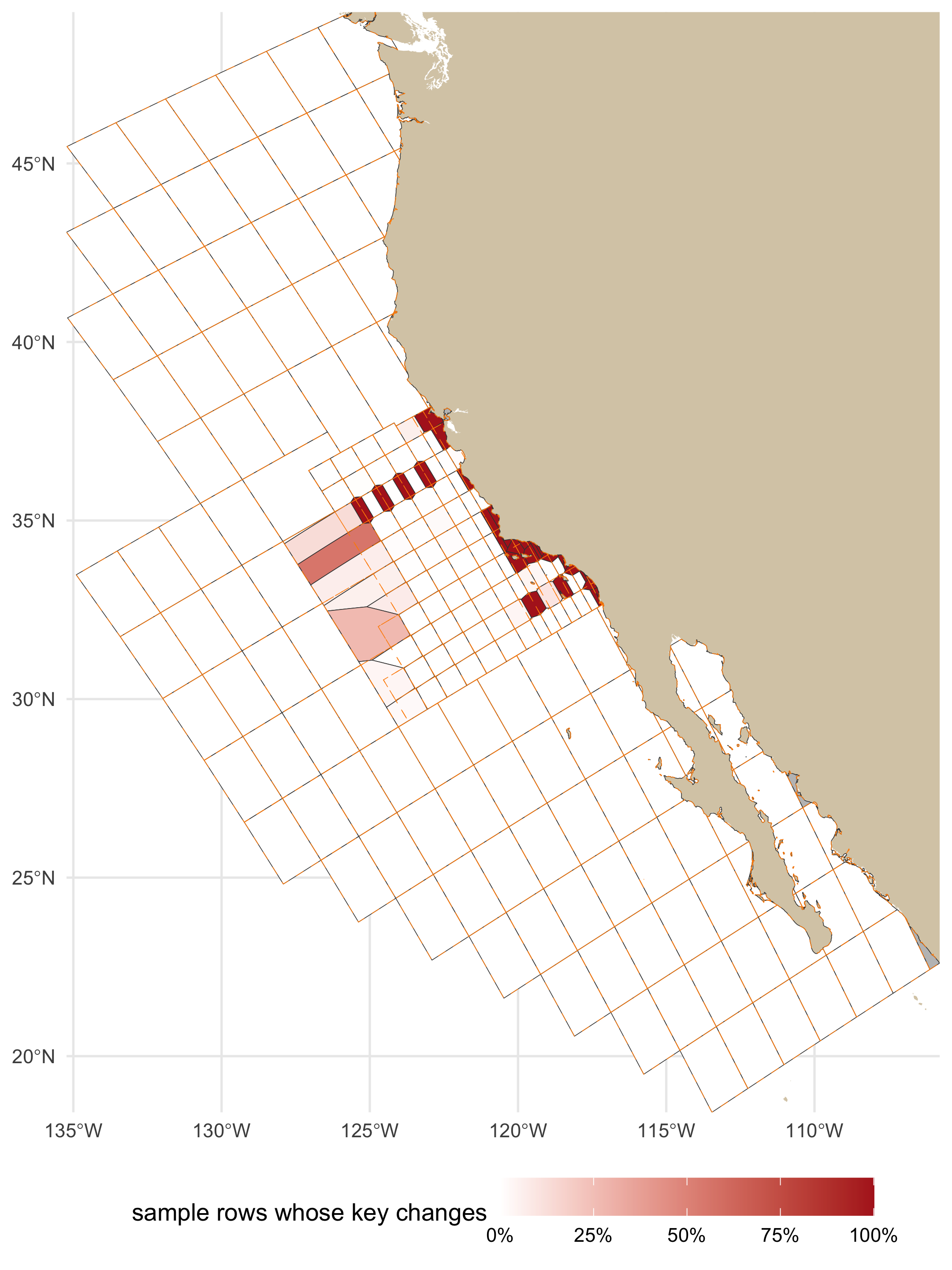
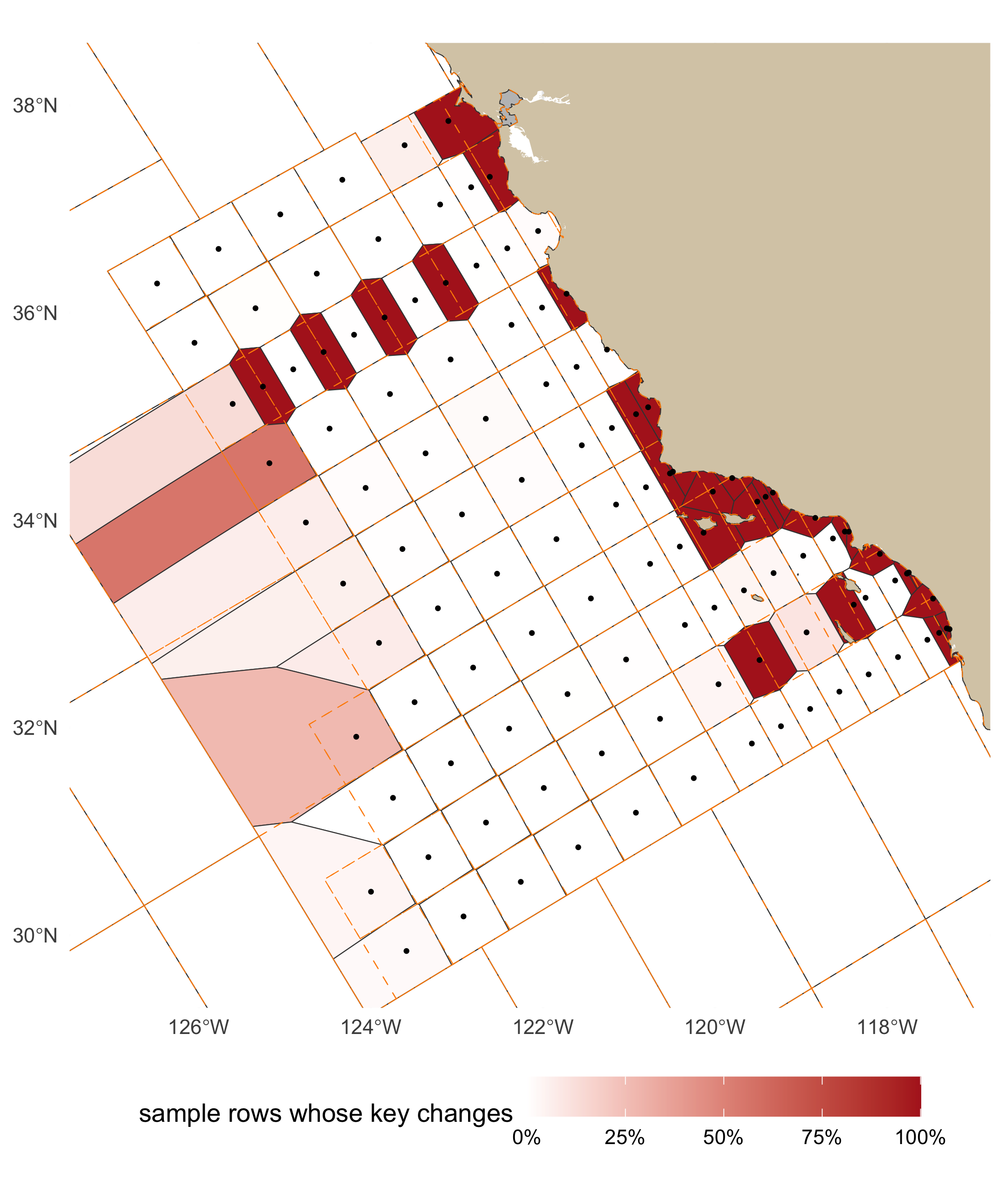
renamed. The change is inside the official pattern, and concentrated inshore, where the lattice
and the stations disagree (@tbl-zone-change, @fig-change-full): the offshore station cells are
the previous lattice cells almost unchanged, and the kept cells do not change at all
(@tbl-kept), which is why the share before 1984, when most of the sampling beyond the pattern
was done, is the smaller one.
```{r}
#| label: tbl-zone-change
#| tbl-cap: "Gate 5: `sample` rows by the zone of their shipped cell, and the share whose key changes."
by_zone |> transmute(zone = zone_key, rows = fmt(rows), `key changes` = fmt(changed), share = pct(share)) |> knitr::kable(align = "lrrr")
```
```{r}
#| label: fig-change-full
#| fig-cap: "Gate 5, full extent: each shipped cell coloured by the share of the `sample` rows now in it whose `grid_key` changes (white: none; grey: fewer than 20 rows, where a share says little). The previous grid's edges are dashed."
#| fig-height: 8
#| fig-width: 6
#| dpi: 180
chg <- dbGetQuery(con, "
  SELECT key_a AS grid_key, count(*) AS n, count(*) FILTER (WHERE key_a IS DISTINCT FROM key_now) AS changed,
         count(*) FILTER (WHERE key_a_main IS DISTINCT FROM key_now) AS moved
  FROM s_key WHERE key_a IS NOT NULL GROUP BY 1")
cc_chg <- cc_grid |> left_join(chg, by = "grid_key") |> mutate(share = ifelse(coalesce(n, 0) >= 20, changed / n, NA))
p_change <- function(xlim, ylim, lw = 0.15, pts = NULL) {
  g <- ggplot() +
    geom_sf(data = land_lite, fill = LAND_FILL, color = NA) +
    geom_sf(data = cc_chg, aes(fill = share), color = "grey25", linewidth = lw) +
    geom_sf(data = grid, fill = NA, color = "darkorange", linewidth = lw, linetype = "dashed")
  if (!is.null(pts)) g <- g + geom_sf(data = pts, size = 0.5, color = "black")
  g + scale_fill_gradient(low = "white", high = "firebrick", na.value = "grey75", limits = c(0, 1), labels = scales::percent,
                          name = "sample rows whose key changes") +
    coord_sf(xlim = xlim, ylim = ylim, expand = FALSE) +
    theme_minimal(base_size = 11) + theme(legend.position = "bottom", legend.key.width = unit(1.2, "cm")) + labs(x = NULL, y = NULL)
}
p_change(c(bb[["xmin"]], bb[["xmax"]]), c(bb[["ymin"]], bb[["ymax"]]))
```
```{r}
#| label: fig-change-pattern
#| fig-cap: "Gate 5, the official pattern (lines 60 to 93.4, out to station 120): the same shares. Offshore cells are the previous lattice cells nearly unchanged; the keys that change are inshore of station 60 and on line 66.7. The kept cells around the pattern are white: their edges did not move."
#| fig-height: 7.2
#| fig-width: 6
#| dpi: 180
p_change(c(-127.5, -116.8), c(29.3, 38.6), lw = 0.2, pts = filter(A_site, gen_source == "official"))
```
**Stations split by a cell edge.** A station's occupations scatter around its position, so a
station near an edge has rows on both sides. @tbl-split counts, per grid, the stations (a
`site_key`, with 20 or more `sample` rows) with under 90% of their rows in one cell.
```{r}
#| label: tbl-split
#| tbl-cap: "Gate 5: stations (`site_key`, at least 20 `sample` rows) whose rows are split across cells: stations with under 90% of their rows in their modal cell, and the rows outside it, under each grid; for all stations and for the 113 official ones."
sta_sql <- "printf('%05.1f %05.1f',
  round(try_cast(regexp_extract(trim(site_key), '^(\\S+)', 1) AS DOUBLE), 1),
  round(try_cast(regexp_extract(trim(site_key), '(\\S+)$', 1) AS DOUBLE), 1))"
invisible(dbExecute(con, glue("CREATE OR REPLACE TABLE s_sta AS SELECT *, {sta_sql} AS station FROM s_key WHERE site_key IS NOT NULL")))
off_in <- paste0("'", sprintf("%05.1f %05.1f", st$line, st$station), "'", collapse = ", ")
split_of <- function(k, only_official = FALSE) {
  flt <- if (only_official) glue("AND station IN ({off_in})") else ""
  dbGetQuery(con, glue("
    WITH c AS (SELECT station, {k} AS cell, count(*) AS rows FROM s_sta
               WHERE station IS NOT NULL AND {k} IS NOT NULL {flt} GROUP BY 1, 2),
         m AS (SELECT station, sum(rows) AS n, max(rows) AS top FROM c GROUP BY 1 HAVING sum(rows) >= 20)
    SELECT count(*) AS stations, count(*) FILTER (WHERE top < 0.9 * n) AS split,
           sum(n - top) AS rows_outside, sum(n) AS rows FROM m"))
}
sp <- bind_rows(
  lapply(c(previous = "key_now", shipped = "key_a", `no SCCOOS` = "key_v"), split_of) |> bind_rows(.id = "grid") |> mutate(stations_of = "all"),
  lapply(c(previous = "key_now", shipped = "key_a", `no SCCOOS` = "key_v"), split_of, only_official = TRUE) |> bind_rows(.id = "grid") |> mutate(stations_of = "official"))
sp |> transmute(stations_of, grid, stations = fmt(stations), `split (< 90% in one cell)` = fmt(split),
                `rows outside the modal cell` = glue("{fmt(rows_outside)} of {fmt(rows)} ({pct(rows_outside / rows, 2)})")) |>
  knitr::kable(align = "llrrr")
```
**Historical line 96.7 keys as it always did.** The official pattern ends at line 93.3 and the
nearest kept cells are the line-100 cells of the historical lattice, whose northern edge the
previous grid put at line 95.0, 20 nautical miles beyond line 93.3. Historical line 96.7 lies
south of that edge. A free Voronoi of the stations would have moved the edge to line 96.65 (40
nautical miles out), onto the line itself; confined to the replaced region, the station cells
stop at line 95.0 and every row of line 96.7 stays in its line-100 cell (@tbl-line967).
```{r}
#| label: tbl-line967
#| tbl-cap: "`sample` rows on historical line 96.7 by the line of the cell they key to, under the previous and the shipped grid, before and from 1984 (expected: every row in a line-100 cell under both)."
l967 <- dbGetQuery(con, "
  SELECT era,
         count(*) FILTER (WHERE key_now LIKE '%-ln100_hist') AS prev_ln100_hist,
         count(*) FILTER (WHERE key_now LIKE '%-ln93.3')     AS prev_ln93_3,
         count(*) FILTER (WHERE key_a LIKE '%-ln100_hist')   AS shipped_ln100_hist,
         count(*) FILTER (WHERE key_a LIKE '%-ln93.3')       AS shipped_ln93_3,
         count(*) AS rows
  FROM s_sta WHERE station LIKE '096.7 %' AND key_a IS NOT NULL GROUP BY 1 ORDER BY 1")
l967_split <- dbGetQuery(con, "
  WITH c AS (SELECT station, key_a AS cell, count(*) AS rows FROM s_sta WHERE station LIKE '096.7 %' AND key_a IS NOT NULL GROUP BY 1, 2),
       m AS (SELECT station, sum(rows) AS n, max(rows) AS top FROM c GROUP BY 1 HAVING sum(rows) >= 20)
  SELECT count(*) AS stations, count(*) FILTER (WHERE top < 0.9 * n) AS split, sum(n - top) AS rows_outside FROM m")
bind_rows(l967, summarize(l967, era = "all", across(-era, sum))) |>
  transmute(era, rows = fmt(rows), `previous: line-100 cells` = fmt(prev_ln100_hist), `previous: line-93.3 cells` = fmt(prev_ln93_3),
            `shipped: line-100 cells` = fmt(shipped_ln100_hist), `shipped: line-93.3 cells` = fmt(shipped_ln93_3)) |>
  knitr::kable(align = "lrrrrr")
l967_prev_split <- dbGetQuery(con, "
  WITH c AS (SELECT station, key_now AS cell, count(*) AS rows FROM s_sta WHERE station LIKE '096.7 %' AND key_now IS NOT NULL GROUP BY 1, 2),
       m AS (SELECT station, sum(rows) AS n, max(rows) AS top FROM c GROUP BY 1 HAVING sum(rows) >= 20)
  SELECT count(*) FILTER (WHERE top < 0.9 * n) AS split FROM m")
l967_changed <- dbGetQuery(con, "SELECT count(*) AS n FROM s_sta WHERE station LIKE '096.7 %' AND key_a IS DISTINCT FROM key_now")$n
cat(glue("line 96.7: {l967_split$stations} stations with 20 or more rows; with under 90% of their rows in one cell: ",
         "{l967_split$split} under the shipped grid, {l967_prev_split$split} under the previous one ",
         "(a station whose occupations straddle an edge between two line-100 cells, the same edge in both); ",
         "rows on line 96.7 whose key changes: {l967_changed}"), "\n")
```
### Gate 6: the variant without SCCOOS cells {#sec-gate6}
The headline numbers of the variant (@sec-variant) are the `no SCCOOS` column of @tbl-headline.
Its `r rv_$cells` cells are the shipped ones except near the nine SCCOOS stations
(@fig-variant): `r fmt(tot$v_changed)` of `r fmt(tot$n)` rows change key against the previous
grid (`r pct(tot$v_changed / tot$n)`; shipped `r pct(tot$a_changed / tot$n)`), and each SCCOOS
station shares the cell of its nearest ROS station.
### `calcofi_dic` and `calcofi_phytoplankton` carry no `grid_key` {#sec-dic}
In v2026.10.01 `grid_key` is NULL on almost every `calcofi_dic` row and on every
`calcofi_phytoplankton` row (@tbl-agree).
```{r}
#| label: tbl-dic
#| tbl-cap: "`sample` rows of the two datasets the release leaves ungridded: with a position, in a cell of each grid, carrying a `grid_key`, and (DIC) parented to a bottle cast."
dbGetQuery(con, "
  SELECT dataset_key, count(*) AS rows, count(longitude) AS with_position, count(key_now) AS in_a_previous_cell,
         count(key_a) AS in_a_shipped_cell, count(grid_key) AS released_with_grid_key,
         count(parent_sample_key) AS parented_to_a_cast,
         count(*) FILTER (WHERE (grid_key IS NULL) = (parent_sample_key IS NULL)) AS key_null_iff_no_parent,
         count(cruise_key) AS with_cruise_key
  FROM s_key WHERE dataset_key IN ('calcofi_dic', 'calcofi_phytoplankton') GROUP BY 1 ORDER BY 1") |>
  knitr::kable(format.args = list(big.mark = ","))
```
**DIC is an ingest gap, not positions outside the grid.** Every DIC row has a position and every
position falls in a cell, under either grid. `ingest_calcofi_dic.qmd` never calls
`assign_grid_key()`: its `sample` projection takes `grid_key` (and `cruise_key`, `order_occ`) from
the matched bottle cast (`c.grid_key` after `LEFT JOIN casts c ON d.cast_id = c.cast_id`), and it
mints a `calcofi_dic:bottle:*` row only for a Niskin `calcofi_bottle` does not already publish,
which are almost all rows with no matched cast. So the key is NULL exactly where there is no
parent cast (the `key_null_iff_no_parent` column). The ingest has since been changed (2026-10-04,
RELEASES.md "DIC: every sample with a position carries a `grid_key`") to key each sample by its
own position, keeping a matched cast's key where there is one. That last clause meets the new
release gate: `check_grid_key_assignment()` stops on a row whose key is not the cell its own
position is in, and a cast-matched DIC sample taken a little off its cast's position can carry
the cast's cell (1 of the 6 in the previous grid). Either the ingest keys every sample by its own
position, or the gate is told which rows inherit a key. `calcofi_phytoplankton` is region-pooled:
its positions are region centroids, and it is ungridded by design.
### The gates, in one table {#sec-gate-table}
```{r}
#| label: tbl-gates
#| tbl-cap: "The six gates on the shipped grid, and the kept-cell rule, measured on v2026.10.01."
ok <- function(x) ifelse(x, "pass", "FAIL")
gates <- tribble(
  ~gate, ~result, ~number, ~status,
  "1. no sample loses its cell", "sample rows with a previous cell and no shipped cell",
    glue("{nrow(lost)} lost ({nrow(gained)} gained)"), ok(nrow(lost) == 0),
  "2a. every official station in its own cell", "stations / sites inside their own cell",
    glue("{sum(sta_key == st$grid_key)} of {nrow(st)} / {sum(site_key == cc_grid_ctrs$grid_key)} of {nrow(cc_grid_ctrs)}"),
    ok(all(sta_key == st$grid_key) && all(site_key == cc_grid_ctrs$grid_key)),
  "2b. every station cell in one piece", "station cells in several pieces; pockets joined to a neighbouring station cell; kept cells in several pieces (previous grid)",
    glue("{n_multi_off} ({paste(cc_grid$grid_key[np_a > 1 & cc_grid$sta_source == 'official'], collapse = ', ')}: {round(sum(cs$area_km2[1]), 1)} km², {sum(cs$rows[1])} sample rows); ",
         "{nrow(b_ship$pockets)}; {n_multi_kept} ({sum(np_v1[kept_keys] > 1)})"),
    ifelse(n_multi_off == 0, "pass", ifelse(all(cc_grid$grid_key[np_a > 1 & cc_grid$sta_source == "official"] %in% cs$grid_key), "pass but 1, reported", "FAIL")),
  "2c. a kept cell holds what it held", "rows whose previous cell is kept: key changes",
    glue("{kept_rows$key_changes} of {fmt(kept_rows$rows)}"), ok(kept_rows$key_changes == 0),
  "3. the crosswalk covers every previous key", "previous keys present; shares summing to one within 1e-6; smallest sum; kept cells with an identity row",
    glue("{sum(xp$n > 0)} of {nrow(xp)}; {sum(abs(xp$frac - 1) <= 1e-6)}; {round(min(xp$frac), 4)}; {nrow(xw_id)} of {length(kept_keys)}"),
    ok(all(xp$n > 0) && all(xp$frac <= 1 + 1e-6) && min(xp$frac) >= 0.95),
  "4. R and DuckDB assign the same key", "differences over sample positions, cell vertices and edge midpoints",
    glue("{sum(g4_tbl[['R ≠ DuckDB']])} of {fmt(nrow(g4))} ({fmt(sum(g4$n_cells >= 2))} on a shared edge)"),
    ok(sum(g4_tbl[["R ≠ DuckDB"]]) == 0 && sum(g4_gate$n_wrong) == 0),
  "5. key changes split at 1984 and by dataset", "rows whose key changes: before 1984 / from 1984 / all",
    glue("{pct(e$share[e$era == era_lv[1]])} / {pct(e$share[e$era == era_lv[2]])} / {pct(tot$a_changed / tot$n)}"), "reported",
  "6. the variant without SCCOOS cells", "cells; rows whose key changes; rows losing their cell",
    glue("{rv_$cells}; {pct(tot$v_changed / tot$n)}; {sum(g1$lost_variant)}"), "reported")
knitr::kable(gates)
```
## The climatology and the stations a cell holds {#sec-climatology}
The climatology (`build_climatology()`, calcofi4db ≥ 4.8.0) is keyed on the **station**
(`sample.site_key`), not the cell, so no grid changes a climatology mean; `grid_key` rides on
each row only as the station's modal cell. Two measures, on the climatology's own inputs
(`calcofi_bottle`, `calcofi_ctd-cast`, `calcofi_dic` samples with a `site_key`,
`r CLIM_YR[1]`–`r CLIM_YR[2]`):
- **cells × month with ≥ 3 cruises**, the grain a cell-keyed baseline (or a map consumer) has;
- **climatology rows whose `grid_key` label would change**: the station's modal cell under each
grid, joined to the release's `climatology` rows.
```{r}
#| label: tbl-climatology
#| tbl-cap: "Effect on the climatology grain: cell × calendar month with at least 3 distinct cruises (1993–2013, climatology input datasets), and climatology rows whose modal-cell label would change."
clim_in <- "dataset_key IN ('calcofi_bottle', 'calcofi_ctd-cast', 'calcofi_dic') AND site_key IS NOT NULL
            AND year(datetime) BETWEEN {CLIM_YR[1]} AND {CLIM_YR[2]}"
cells_month <- function(k) dbGetQuery(con, glue("
  SELECT count(*) n FROM (
    SELECT {k}, month(datetime) m FROM s_key WHERE {k} IS NOT NULL AND {glue(clim_in)}
    GROUP BY ALL HAVING count(DISTINCT cruise_key) >= 3)"))$n
modal <- function(k) glue("
  SELECT dataset_key, site_key, mode({k}) AS cell FROM s_key WHERE {glue(clim_in)} GROUP BY ALL")
clim_change <- function(k) dbGetQuery(con, glue("
  WITH now AS ({modal('key_now')}), opt AS ({modal(k)})
  SELECT count(*) AS n_rows, count(*) FILTER (WHERE now.cell IS DISTINCT FROM opt.cell) AS changed,
         count(DISTINCT (c.dataset_key, c.site_key)) FILTER (WHERE now.cell IS DISTINCT FROM opt.cell) AS stations
  FROM climatology c JOIN now USING (dataset_key, site_key) JOIN opt USING (dataset_key, site_key)"))
# the release's own label against the recomputed modal (they differ only where obs weighting differs)
lab <- dbGetQuery(con, glue("
  WITH now AS ({modal('key_now')})
  SELECT count(*) n, count(*) FILTER (WHERE c.grid_key IS NOT DISTINCT FROM now.cell) same
  FROM climatology c JOIN now USING (dataset_key, site_key)"))
ca <- clim_change("key_a"); cv <- clim_change("key_v"); cb <- clim_change("key_b")
clim_tbl <- tibble(
  grid = c("previous", "shipped", "no SCCOOS", "B", "C"),
  `cells × month with ≥ 3 cruises` = c(cells_month("key_now"), cells_month("key_a"), cells_month("key_v"), cells_month("key_b"), cells_month("key_now")),
  `climatology rows relabelled` = c("", glue("{fmt(ca$changed)} of {fmt(ca$n_rows)} ({ca$stations} stations)"),
                                    glue("{fmt(cv$changed)} of {fmt(cv$n_rows)} ({cv$stations} stations)"),
                                    glue("{fmt(cb$changed)} of {fmt(cb$n_rows)} ({cb$stations} stations)"), "0"))
knitr::kable(clim_tbl)
```
The recomputed modal cell matches the released `climatology.grid_key` on
`r fmt(lab$same)` of `r fmt(lab$n)` rows (the release takes the mode over `obs` rows, this over
samples).
### Cells that hold several stations, in the data
```{r}
#| label: tbl-stations-per-cell
#| tbl-cap: "Cells holding two or more distinct CTD stations (`calcofi_ctd-cast` `site_key`, each occupied on at least 3 cruises since 2004 and counted in the cell most of its casts fall in), under each grid."
# a station's cell is the cell most of its casts fall in (casts scatter within ~2 nmi of the
# position, so a station near an edge has casts on both sides)
sk <- dbGetQuery(con, "
  SELECT site_key, mode(key_now) AS key_now, mode(key_a) AS key_a, mode(key_v) AS key_v, mode(key_b) AS key_b
  FROM s_key WHERE dataset_key = 'calcofi_ctd-cast' AND site_key IS NOT NULL AND year(datetime) >= 2004
  GROUP BY site_key HAVING count(DISTINCT cruise_key) >= 3")
# normalize the station label: source forms differ ('093.3 026.4', '93.3    26.4', '090.0 27.76')
sk <- sk |> mutate(
  st_line = as.numeric(sub("^\\s*(\\S+)\\s+.*$", "\\1", site_key)),
  st_sta  = as.numeric(sub("^.*\\s+(\\S+)\\s*$", "\\1", site_key)),
  station = sprintf("%.1f %.1f", round(st_line, 1), round(st_sta, 1))) |>
  distinct(station, .keep_all = TRUE)
multi <- function(k) sk |> filter(!is.na(.data[[k]])) |> count(cell = .data[[k]]) |> filter(n >= 2)
mrow <- function(k) c(nrow(multi(k)), sum(multi(k)$n), max(c(0, multi(k)$n)))
mt <- sapply(c(previous = "key_now", shipped = "key_a", `no SCCOOS` = "key_v", B = "key_b", C = "key_now"), mrow)
tibble(grid = colnames(mt), `cells with ≥ 2 stations` = mt[1, ], `stations in such cells` = mt[2, ],
       `most stations in one cell` = mt[3, ]) |> knitr::kable()
```
In the shipped grid a cell still holds two stations in the data where a station that is not in
the official table (†), or casts labelled with an official station but taken nearer another, was
occupied on 3 or more cruises since 2004 (@tbl-a-multi): those stations key to the nearest
official station.
```{r}
#| label: tbl-a-multi
#| tbl-cap: "Shipped cells holding two or more CTD stations in the data (each occupied on ≥ 3 cruises since 2004, in the cell most of its casts fall in); stations not in the official table are marked †."
off_keys <- sprintf("%.1f %.1f", st$line, st$station)
sk |> filter(!is.na(key_a)) |>
  group_by(key_a) |> filter(n() >= 2) |>
  summarize(n = n(), stations = paste(ifelse(station %in% off_keys, station, paste0(station, " †")), collapse = "; ")) |>
  arrange(desc(n), key_a) |> rename(grid_key = key_a) |> knitr::kable()
```
## Headline {#sec-headline}
```{r}
#| label: tbl-headline
#| tbl-cap: "The shipped grid beside the previous grid, the variant without SCCOOS cells and the two repairs, on v2026.10.01."
parts_v_after <- flag_slivers(split_parts(transmute(V, grid_key)), st_transform(b_var$ctrs, CRS_M))
V_site <- b_var$ctrs
V_off  <- off_line_km(st_coordinates(V_site)[, 1], st_coordinates(V_site)[, 2], V_site$sta_lin)
n_multi_parts <- function(p) sum(p$part == 1 & p$n_parts > 1)
row_share <- function(col) pct(tot[[col]] / tot$n)
area_rng  <- function(a) glue("{fmt(min(a), 1)} to {fmt(max(a))}")
hl <- tibble(
  ` ` = c("cells", "cells in more than one piece", glue("sites > {OFF_KM} km off their line"),
          "sliver parts touching another cell", "cells holding ≥ 2 official stations", "cell area (km²)", "station cell area (km²)",
          "sample rows that lose their cell", "sample rows whose grid_key changes", "  of which a real move (not a rename)",
          "cells × month with ≥ 3 cruises (1993–2013)", "climatology rows relabelled", "vertices"),
  previous = c(nrow(grid), n_multi_parts(parts_now), sum(grid$off_km > OFF_KM), sum(parts_now$sliver & parts_now$touches_other),
            sum(n_per_cell >= 2), area_rng(as.numeric(st_area(gm)) / 1e6), "", "", "", "", clim_tbl[[2]][1], "", fmt(n_vertices(cc_grid_v1))),
  shipped = c(nrow(A), n_multi_parts(parts_a_after), sum(A_off > OFF_KM), sum(parts_a_after$sliver & parts_a_after$touches_other),
        sum(n_per_cell_a >= 2), area_rng(A$area_km2), area_rng(A$area_km2[A$gen_source == "official"]),
        sum(g1$lost), row_share("a_changed"), row_share("a_moved"),
        clim_tbl[[2]][2], clim_tbl[[3]][2], fmt(n_vertices(cc_grid))),
  `no SCCOOS` = c(nrow(V), n_multi_parts(parts_v_after), sum(V_off > OFF_KM), sum(parts_v_after$sliver & parts_v_after$touches_other),
        sum(table(cc_grid_key(st$longitude, st$latitude, b_var$grid)) >= 2), area_rng(V$area_km2),
        area_rng(V$area_km2[b_var$grid$sta_source == "official"]), sum(g1$lost_variant),
        row_share("v_changed"), row_share("v_moved"), clim_tbl[[2]][3], clim_tbl[[3]][3], fmt(n_vertices(b_var$grid))),
  B = c(nrow(B), n_multi_parts(parts_b_after), sum(B_off > OFF_KM), sum(parts_b_after$sliver & parts_b_after$touches_other),
        sum(table(first_hit(stp, B)) >= 2), area_rng(as.numeric(st_area(B)) / 1e6), "", "", row_share("b_changed"), row_share("b_changed"),
        clim_tbl[[2]][4], clim_tbl[[3]][4], ""),
  C = c(nrow(grid), n_multi_parts(parts_now), sum(!c_ok), sum(parts_now$sliver & parts_now$touches_other),
        sum(n_per_cell >= 2), area_rng(as.numeric(st_area(gm)) / 1e6), "", "0", "0.0%", "0.0%", clim_tbl[[2]][5], "0", fmt(n_vertices(cc_grid_v1))))
hl <- mutate(hl, across(everything(), as.character))
knitr::kable(hl)
```
The shipped grid's `r hl$shipped[2]` cells in more than one piece, its `r hl$shipped[4]` sliver
parts and its `r sum(A_off > OFF_KM)` sites more than `r OFF_KM` km off their line
(`r sum(A_off > OFF_KM & A_site$gen_source == "official")` of them official stations) are all kept
cells, which are the previous cells as they were (@tbl-multipart), but for the one station cell of
@tbl-cases.
## What shipped, and what is still a question {#sec-recommendation}
**Shipped** (Ben, 2026-10-04): one cell per official station, SCCOOS stations included, as the
Voronoi of the 113 official positions confined to the previous cells it replaces; the previous
cells beyond the official pattern kept as they were; and a key crosswalk. It is the only option
that fixes both defects at the source: every official site *is* an official position, which
`+proj=calcofi` reproduces to within `r round(max(st$dist_m))` m; no station cell is a remnant
of an idealized lattice; and no cell holds two official stations (the previous grid:
`r hl$previous[5]` cells), which ends the station mixing that #86 and the climatology work routed
around with `site_key`. Option B removes the slivers but keeps the nominal lattice
(`r hl$B[3]` sites still more than `r OFF_KM` km off their line, `r hl$B[5]` cells still holding
several official stations); Option C moves the dots and nothing else, and cannot place
`r sum(!c_ok)` sites at all because their own line misses their cell.
The price is `r hl$shipped[9]` of `sample` rows changing `grid_key`, `r hl$shipped[10]` moving to
a different cell rather than a renamed one (@tbl-per-dataset), all of them inside the official
pattern, and `r fmt(ca$changed)` of `r fmt(ca$n_rows)` climatology rows (`r ca$stations`
stations) taking a new modal-cell label; the climatology means do not move (they are keyed on
`site_key`), and the cell-month grain with three or more cruises grows from
`r clim_tbl[[2]][1]` to `r clim_tbl[[2]][2]` because the inshore stations stop sharing cells.
**Choices the build makes that the 2026-10-08 meeting has not seen** (each is one argument or one
rule of `cc_grid_build()` / `cc_grid_land_prep()`, and can change without touching anything else):
1. **Keys.** A cell is named for its station, `st{station}-ln{line}`, decimals as listed
(`st26.7-ln93.3`, `st26.4-ln93.4`, `st43.5-ln81.7`); a kept cell keeps its previous key.
2. **SCCOOS stations get cells** (@tbl-option-a-cells: `r fmt(min(A$area_km2[which(A$sta_type == "SCCOOS")]), 1)`
to `r fmt(max(A$area_km2[which(A$sta_type == "SCCOOS")]))` km²), six of the nine on lines of their
own (81.7, 85.4, 86.8, 88.5, 91.7, 93.4; the rosette station 81.8 46.9 is alone on its line
too), so a section along line 93.3 no longer includes 93.4 26.4. The variant (@sec-variant) is
the alternative.
3. **Attributes.** `shore`: nearshore at station ≤ 60. `pattern`: standard on lines ≥ 76.7,
extended north of it, historical for a kept cell (one kept cell, `st45-ln60`, stays
`extended`). `spacing`: the nominal class 5 / 10 / 20, not the measured distance to the next
station. `zone` = `{shore}-{pattern}`.
4. **Kept cells are the previous cells** (Ben, 2026-10-04): the `r length(kept_keys)` previous
cells whose label is more than 20 nautical miles outside the official pattern keep their own
boundaries and their pieces (`r n_multi_kept` are in several). No `sample` row leaves one
(@tbl-kept).
5. **The station cells are confined to the previous cells they replace** (Ben, 2026-10-04), so
the outer station cells stop where the previous lattice stopped them: line 95.0 in the south,
and the previous cells' outer edges to the north and offshore. Three replaced cells are
historical ones just beyond the pattern (`r paste(prevt$grid_key[prevt$fate == "replaced" & prevt$sta_pattern == "historical"], collapse = ", ")`):
the outer station cells take their water, up to `r fmt(max(A$area_km2[A$gen_source == "official"]))` km².
6. **A historical cast** inside the replaced region keys to the nearest official station's cell
(90.0 32, 1959–84, keys to
`r cc_grid_key(cc_calcofi_to_lonlat(90, 32)$longitude, cc_calcofi_to_lonlat(90, 32)$latitude)`),
and to its kept cell beyond. @tbl-a-multi lists the stations this affects since 2004.
7. **A kept cell's site** is its label, else the previous cell's centre
(`r sum(prevt$site_at == "centre", na.rm = TRUE)` cells, label on land), else a point on the
cell (`r sum(prevt$site_at == "water", na.rm = TRUE)`).
8. **The coastline** is OpenStreetMap's, islets under 1 km² dropped, pulled back 300 m and
simplified to 100 m; cells therefore reach up to 300 m onto land, and `area_km2` includes that
strip. Water between the previous grid's coarser coastline and this one joins the cell it is
nearest to (`r fmt(sum(prevt$gap_km2))` km² to the kept cells).
9. **Pockets** join the neighbouring station cell with the longest shared water edge
(@tbl-pockets), never a kept cell.
10. **Previous cells that overlap** (along the line 93.3 / line 100 boundary, under 1 km² in all):
the overlap is the cell whose key sorts first, which is the cell `cc_grid_key()` gives a
position there in the previous grid.
**Still open:**
- the one piece of the replaced region no station cell reaches (@tbl-cases): Tomales Bay stays
with `st53-ln60` as a detached part, because joining it to the kept cell it opens into would
move a kept cell's boundary;
- whether the kept cells should stay in pieces (@tbl-multipart): keeping them literal is what
keeps every historical key, and `r n_multi_kept` of them are multi-part as
`r sum(np_v1[kept_keys] > 1)` already were;
- which 9 stations of line 66.7 are the 113-only infill (the page does not say; all 11 have a
cell);
- whether `st45-ln60` (San Francisco Bay and its approaches) should exist;
- whether the Navy stations need anything on a map.
```{r}
#| label: cleanup
close_duckdb(con_g)
close_duckdb(con)
```