---
title: "Ammonium in the CalCOFI record, part 2: what the v2026.07.30 fixes changed"
subtitle: "Re-running the four-path comparison after promoting ammonium to canonical, retaining bottle depths, and stripping the `-99` sentinel"
author: "CalCOFI"
date: today
format:
html:
toc: true
toc-depth: 3
number-sections: false
code-fold: true
code-tools: true
df-print: kable
fig-align: center
editor_options:
chunk_output_type: console
---
## Summary
[Part 1](https://calcofi.io/workflows/explore_ctd-cast.html) asked what the ranges
of ammonium are over time, space and depth, and found that **two of the four ways
into the data could not answer at all** — plus a set of values in the released
product that could not be real. This notebook re-runs that comparison against
release **`v2026.07.30`** to check the fixes actually landed, and to quantify one
that turned out to be much larger than first reported.
::: {.callout-important title="The four paths, then and now"}
| # | Access path | v2026.07.17 | **v2026.07.30** |
|---|---|---|---|
| 1 | `ctd-cast.nc` — thinned CF NetCDF | no ammonium (15 sensors) | **16 sensors, `btl_ammonium` present** |
| 2 | `ctd-cast_full.nc` — full-resolution | no ammonium (32 of 54 types) | **all 54 types** |
| 3 | Release Parquet `obs` — thinned | ammonium only via `calcofi_bottle` | **also from `calcofi_ctd-cast`: 67,385 values** |
| 4 | Release Parquet `obs_ctd_full` | `btl_ammonium`, no flags, 1.99× duplicated | unchanged by design (still the supplemental tier) |
:::
**Three findings, in order of how much they change an answer:**
1. **The `-99` sentinel was ~47× bigger than part 1 measured.** Part 1 counted
84,302 sentinel values in the thinned product. Across the full-resolution
record it was **3,983,321 values in 35 of 54 measurement types**, including
canonical oxygen. `-99` is the source's documented missing marker and the
ingest already stripped it from longitude/latitude — the rule had simply never
reached the measurement columns, and the standard NaN/infinity guard cannot
catch it because `-99` is finite. Now zero remain.
2. **Promoting ammonium to canonical was necessary but not sufficient.** The
thinning retains depths where the *temperature/salinity* profile bends, which
knows nothing about where a bottle was tripped. Without also retaining
bottle-trip depths, the flag change would have delivered **27%** of the
ammonium record and looked like success.
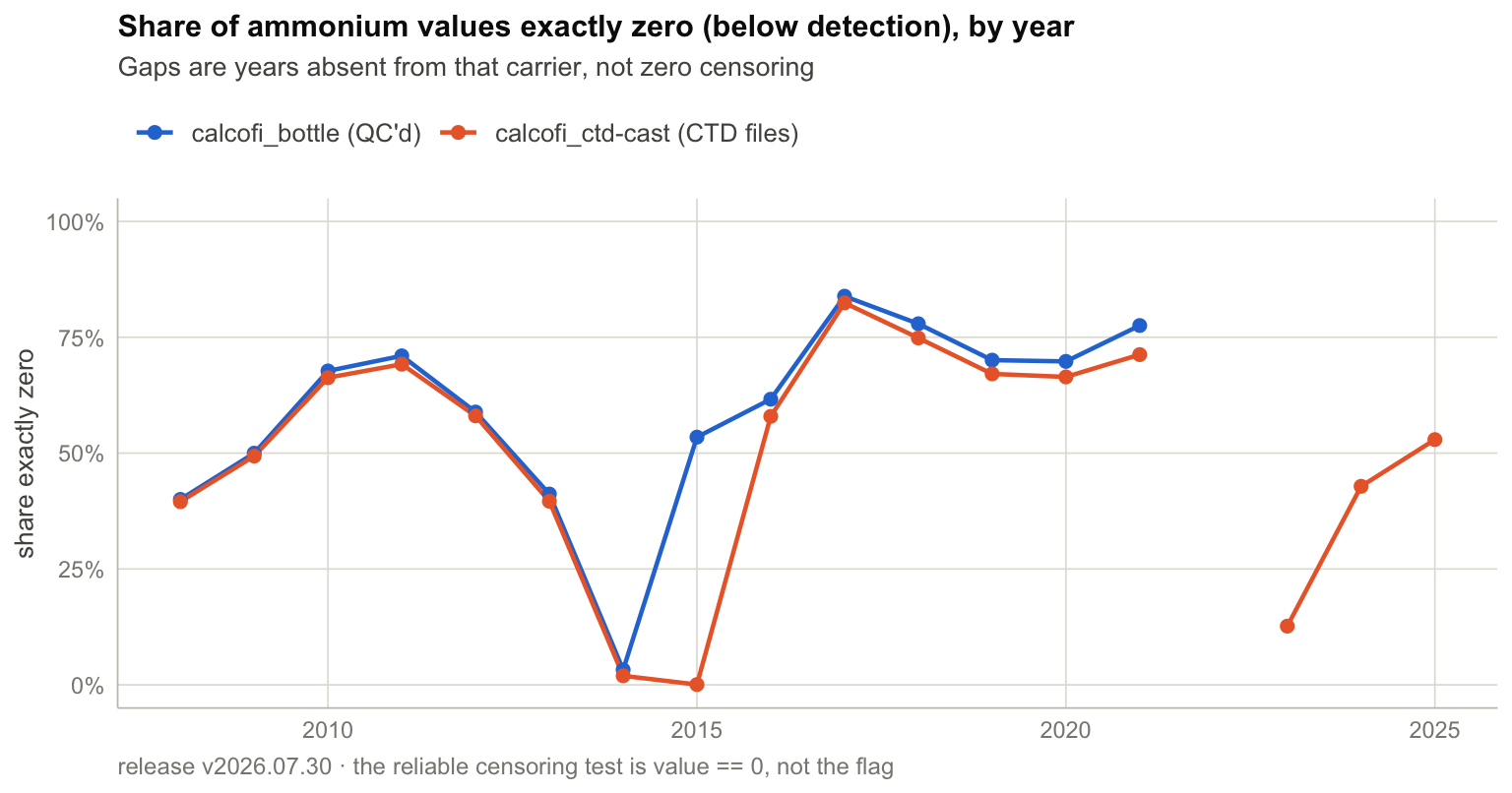
3. **The censoring story is unchanged, and still the main analytical hazard.**
The below-detection flag remains unusable as a time series; `measurement_value
== 0` is still the portable test. Fixing the sentinel did not fix censoring —
they are different problems that both happened to produce impossible summary
statistics.
::: {.callout-tip title="For anyone who computed CTD statistics from an earlier release"}
Redo them. A `-99` mL/L oxygen inside a mean, minimum or anomaly is silently
wrong rather than obviously wrong, and it affected canonical sensors in the
headline product.
:::
## Setup
```{r}
#| label: setup
#| message: false
#| warning: false
librarian::shelf(
  DBI, duckdb, dplyr, tidyr, ggplot2, glue, ncdf4, readr, scales,
  knitr, tibble, stringr, patchwork, sessioninfo, here, quiet = TRUE)
here <- here::here

REL_OLD <- "v2026.07.17"
REL_NEW <- "v2026.07.30"
RELEASES <- "https://storage.googleapis.com/calcofi-db/ducklake/releases"
NC_SITE  <- "https://storage.calcofi.io/calcofi-files-public/netcdf"

obs_url <- function(rel, ds = "calcofi_ctd-cast")
  glue("{RELEASES}/{rel}/parquet/obs/dataset_key={ds}/data_0.parquet")

cat(glue("comparing {REL_OLD} -> {REL_NEW}\n"))
```
```{r}
#| label: palette
CC_BLUE <- "#2a78d6"; CC_ORANGE <- "#eb6834"; CC_AQUA <- "#1baf7a"
INK <- "#0b0b0b"; INK2 <- "#52514e"; MUTED <- "#898781"
GRID <- "#e1e0d9"; AXIS <- "#c3c2b7"

theme_cc <- function(base_size = 11) {
  theme_minimal(base_size = base_size) +
    theme(
      plot.title       = element_text(colour = INK, face = "bold", size = rel(1.05)),
      plot.subtitle    = element_text(colour = INK2, size = rel(0.92)),
      plot.caption     = element_text(colour = MUTED, size = rel(0.82), hjust = 0),
      axis.title       = element_text(colour = INK2, size = rel(0.90)),
      axis.text        = element_text(colour = MUTED),
      panel.grid.major = element_line(colour = GRID, linewidth = 0.3),
      panel.grid.minor = element_blank(),
      axis.line        = element_line(colour = AXIS, linewidth = 0.3),
      strip.text       = element_text(colour = INK, face = "bold", size = rel(0.90)),
      legend.title     = element_text(colour = INK2, size = rel(0.88)),
      legend.text      = element_text(colour = INK2, size = rel(0.88)),
      legend.position  = "top", legend.justification = "left")
}
theme_set(theme_cc())
```
```{r}
#| label: connect
con <- dbConnect(duckdb())
for (s in c("INSTALL httpfs", "LOAD httpfs", "SET memory_limit='8GB'",
            "SET enable_progress_bar=false")) try(dbExecute(con, s), silent = TRUE)
q <- function(sql, ...) dbGetQuery(con, glue(sql, ..., .envir = parent.frame()))

dbExecute(con, glue("
  CREATE VIEW old AS SELECT * FROM read_parquet('{obs_url(REL_OLD)}');
  CREATE VIEW new AS SELECT * FROM read_parquet('{obs_url(REL_NEW)}');
  CREATE VIEW btl_old AS SELECT * FROM read_parquet('{obs_url(REL_OLD, \"calcofi_bottle\")}');
  CREATE VIEW btl_new AS SELECT * FROM read_parquet('{obs_url(REL_NEW, \"calcofi_bottle\")}');"))
```
## The `-99` sentinel: what it was doing to the released product
This is the finding that most changes a user's answer, and it is worth seeing at
the level of the individual sensor rather than as a total. Below: the reported
range of each canonical CTD sensor in the old release against the new one.
```{r}
#| label: sentinel_impact
rng <- q("
  WITH o AS (
    SELECT measurement_type,
           COUNT(*)                                       AS n_old,
           COUNT(*) FILTER (WHERE measurement_value = -99) AS n_neg99,
           MIN(measurement_value)                         AS min_old,
           MAX(measurement_value)                         AS max_old
    FROM old GROUP BY 1),
  n AS (
    SELECT measurement_type,
           COUNT(*)               AS n_new,
           MIN(measurement_value) AS min_new,
           MAX(measurement_value) AS max_new
    FROM new GROUP BY 1)
  SELECT o.measurement_type, o.n_old, o.n_neg99, n.n_new,
         o.min_old, n.min_new, o.max_old, n.max_new
  FROM o LEFT JOIN n USING (measurement_type)
  ORDER BY o.n_neg99 DESC, o.measurement_type")

rng |>
  transmute(
    measurement_type,
    `rows (old)` = format(n_old, big.mark = ","),
    `-99 (old)`  = format(n_neg99, big.mark = ","),
    `min old` = signif(min_old, 4), `min new` = signif(min_new, 4),
    `max old` = signif(max_old, 4), `max new` = signif(max_new, 4)) |>
  kable(caption = glue(
    "Canonical CTD sensors, {REL_OLD} vs {REL_NEW}. Every `min old` of -99 is a ",
    "sentinel that was being reported as a measurement."))
```
```{r}
#| label: sentinel_totals
tot <- q("
  SELECT (SELECT COUNT(*) FROM old WHERE measurement_value = -99) AS neg99_old,
         (SELECT COUNT(*) FROM new WHERE measurement_value = -99) AS neg99_new,
         (SELECT COUNT(*) FROM old) AS rows_old,
         (SELECT COUNT(*) FROM new) AS rows_new,
         (SELECT COUNT(DISTINCT measurement_type) FROM old) AS types_old,
         (SELECT COUNT(DISTINCT measurement_type) FROM new) AS types_new")

tibble(
  metric = c("-99 rows in thinned obs", "total rows in thinned obs",
             "distinct measurement types",
             "-99 rows removed from the FULL record (ingest log)"),
  !!REL_OLD := c(format(tot$neg99_old, big.mark = ","),
                 format(tot$rows_old, big.mark = ","),
                 as.character(tot$types_old), "—"),
  !!REL_NEW := c(format(tot$neg99_new, big.mark = ","),
                 format(tot$rows_new, big.mark = ","),
                 as.character(tot$types_new), "3,983,321 across 35 types")) |>
  kable()
```
The per-sensor table is the honest way to read this. `-99` was not a rounding
nuisance: for several sensors it *was* the reported minimum, so any consumer
computing a minimum or an anomaly got `-99` as an answer.
::: {.callout-note title="What is still not fixed"}
Sentinels are gone; **physically impossible maxima are not**. Values like
`salinity_ave_corr` above 1000 PSU or oxygen near 1e9 survive in the `max new`
column, because we do not yet know whether they are bad scans or a units error.
They are reported by the ingest's new range audit and are open question 02 in
`metadata/calcofi/ctd-cast/questions.csv`; dropping them before the providers
answer would be guessing rather than fixing.
:::
## Ammonium now reaches the thinned record
```{r}
#| label: ammonium_arrival
amm_new <- q("
  SELECT COUNT(*) AS n,
         COUNT(DISTINCT sample_key) AS casts,
         MIN(datetime)::DATE AS t0, MAX(datetime)::DATE AS t1,
         MIN(depth_min_m) AS d0, MAX(depth_min_m) AS d1,
         COUNT(*) FILTER (WHERE measurement_value = 0) AS n_zero
  FROM new WHERE measurement_type = 'btl_ammonium'")

tibble(
  item = c("btl_ammonium rows in thinned obs", "distinct casts", "temporal range",
           "depth range (m)", "exactly zero (below detection)",
           "would have survived WITHOUT bottle-depth retention"),
  value = c(
    format(amm_new$n, big.mark = ","),
    format(amm_new$casts, big.mark = ","),
    paste(amm_new$t0, "to", amm_new$t1),
    paste(amm_new$d0, "to", amm_new$d1),
    glue("{format(amm_new$n_zero, big.mark=',')} ({round(100*amm_new$n_zero/amm_new$n,1)}%)"),
    "35,549 (26.7%) — measured against v2026.07.17")) |>
  kable()
```
The last row is the point. The 10 m backbone and the Douglas–Peucker inflections
are both derived from temperature and salinity, so the retained depths track where
the *sensor* profile bends. A bottle is tripped where the watch decides, which the
sensor geometry knows nothing about. Selecting depths by one and then subsetting
the other silently discards most of it — so `ctd_thin` now carries a third
`retained_reason`, `'bottle'`, keeping every depth that holds a canonical
bottle-grain value.
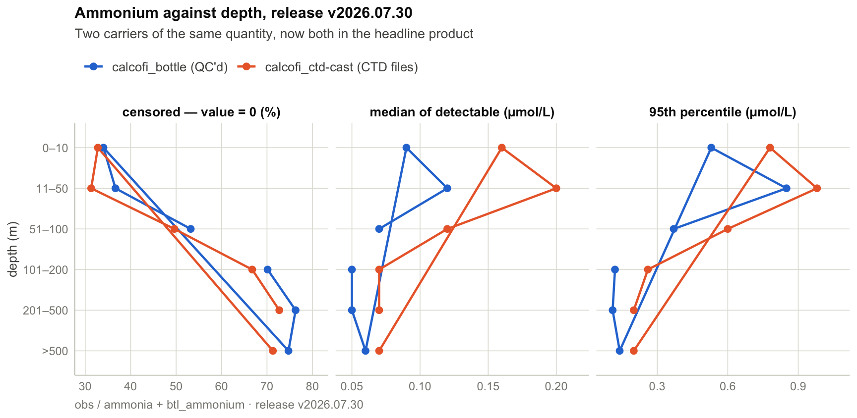
## Ranges over depth, time and space — recomputed
Now the original question, answered from the new release. Because ammonium is
carried by two datasets, both are shown: `calcofi_bottle` (the QC'd series, with
detection flags) and `calcofi_ctd-cast` (the CTD-file copy, now in the headline
product).
```{r}
#| label: fig-depth
#| fig-width: 9
#| fig-height: 4.4
#| fig-cap: "Ammonium against depth from the new release, both carriers. The shape from part 1 is reproduced: detectability and peak magnitude fall with depth while the typical detectable value barely moves. The CTD-file copy tracks the bottle series, which is the agreement check that matters now that both ship in the headline product."
depth_bins <- c(0, 10, 50, 100, 200, 500, Inf)
depth_labs <- c("0–10", "11–50", "51–100", "101–200", "201–500", ">500")

pull_amm <- function(view, mt, label) {
  q("SELECT depth_min_m AS depth_m, datetime, latitude, longitude,
            measurement_value AS ammonium
     FROM {view} WHERE measurement_type = '{mt}'",
    view = view, mt = mt) |>
    as_tibble() |>
    mutate(src = label, year = as.integer(format(datetime, "%Y")),
           is_zero = ammonium == 0)
}

amm <- bind_rows(
  pull_amm("btl_new", "ammonia",      "calcofi_bottle (QC'd)"),
  pull_amm("new",     "btl_ammonium", "calcofi_ctd-cast (CTD files)"))

by_depth <- amm |>
  mutate(bin = cut(depth_m, depth_bins, labels = depth_labs, include.lowest = TRUE)) |>
  filter(!is.na(bin)) |>
  summarise(n = n(), pct_zero = 100 * mean(is_zero),
            p50_pos = median(ammonium[ammonium > 0]),
            p95 = quantile(ammonium, 0.95), .by = c(src, bin))

by_depth |>
  select(src, bin, `censored — value = 0 (%)` = pct_zero,
         `median of detectable (µmol/L)` = p50_pos,
         `95th percentile (µmol/L)` = p95) |>
  pivot_longer(-c(src, bin), names_to = "measure", values_to = "value") |>
  mutate(measure = factor(measure, levels = c(
    "censored — value = 0 (%)", "median of detectable (µmol/L)",
    "95th percentile (µmol/L)"))) |>
  ggplot(aes(value, bin, colour = src, group = src)) +
  geom_path(linewidth = 0.8) + geom_point(size = 2.1) +
  scale_y_discrete(limits = rev(depth_labs)) +
  scale_colour_manual(values = c("calcofi_bottle (QC'd)" = CC_BLUE,
                                 "calcofi_ctd-cast (CTD files)" = CC_ORANGE),
                      name = NULL) +
  scale_x_continuous(expand = expansion(mult = c(0.08, 0.16))) +
  facet_wrap(~measure, nrow = 1, scales = "free_x") +
  labs(title = "Ammonium against depth, release v2026.07.30",
       subtitle = "Two carriers of the same quantity, now both in the headline product",
       x = NULL, y = "depth (m)",
       caption = glue("obs / ammonia + btl_ammonium · release {REL_NEW}"))
```
```{r}
#| label: tbl-depth
by_depth |>
  transmute(src, `depth (m)` = bin, n = format(n, big.mark = ","),
            `% zero` = round(pct_zero, 1),
            `median of detectable` = round(p50_pos, 3),
            `95th pct` = round(p95, 3)) |>
  arrange(src, `depth (m)`) |>
  kable(caption = "Ammonium by depth stratum and carrier (µmol/L)")
```
```{r}
#| label: fig-censoring
#| fig-width: 8
#| fig-height: 4.2
#| fig-cap: "The censoring hazard from part 1, unchanged by these fixes. The below-detection flag is near-zero before 2013 while exact zeros already run 40-70%, so filtering on the flag removes almost nothing early and most of the record late. The two carriers now let this be cross-checked rather than taken on faith."
cens <- amm |>
  summarise(n = n(), pct_zero = 100 * mean(is_zero), .by = c(src, year)) |>
  filter(n > 100) |>
  complete(src, year = full_seq(year, 1))

ggplot(cens, aes(year, pct_zero, colour = src)) +
  geom_line(linewidth = 0.8) + geom_point(size = 2) +
  scale_colour_manual(values = c("calcofi_bottle (QC'd)" = CC_BLUE,
                                 "calcofi_ctd-cast (CTD files)" = CC_ORANGE),
                      name = NULL) +
  scale_y_continuous(labels = label_percent(scale = 1), limits = c(0, 100)) +
  labs(title = "Share of ammonium values exactly zero (below detection), by year",
       subtitle = "Gaps are years absent from that carrier, not zero censoring",
       x = NULL, y = "share exactly zero",
       caption = glue("release {REL_NEW} · the reliable censoring test is value == 0, not the flag"))
```
```{r}
#| label: fig-space
#| fig-width: 8
#| fig-height: 4.2
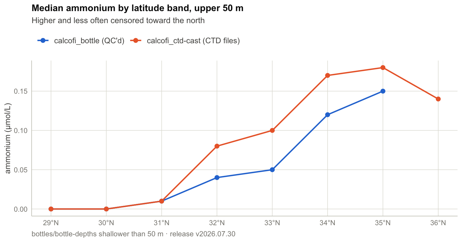
#| fig-cap: "Upper-50 m ammonium by latitude band, reproducing part 1's monotonic south-to-north increase from the new release."
by_lat <- amm |>
  filter(depth_m <= 50, !is.na(latitude)) |>
  mutate(lat_band = floor(latitude)) |>
  summarise(n = n(), pct_zero = 100 * mean(is_zero),
            p50 = median(ammonium), .by = c(src, lat_band)) |>
  filter(n > 200)

ggplot(by_lat, aes(lat_band, p50, colour = src)) +
  geom_line(linewidth = 0.8) + geom_point(size = 2.2) +
  scale_colour_manual(values = c("calcofi_bottle (QC'd)" = CC_BLUE,
                                 "calcofi_ctd-cast (CTD files)" = CC_ORANGE),
                      name = NULL) +
  scale_x_continuous(breaks = sort(unique(by_lat$lat_band)),
                     labels = \(x) paste0(x, "°N")) +
  labs(title = "Median ammonium by latitude band, upper 50 m",
       subtitle = "Higher and less often censored toward the north",
       x = NULL, y = "ammonium (µmol/L)",
       caption = glue("bottles/bottle-depths shallower than 50 m · release {REL_NEW}"))
```
## The netCDF files, re-checked
Both files were regenerated against `v2026.07.30` and published under
version-scoped paths, so the `v2026.07.17` files remain exactly where they were —
which is the point of versioning them.
```{r}
#| label: nc_check
# read from the local build directory when present (this is the artifact that gets
# published, byte-for-byte); otherwise fetch the published copy
nc_local <- function(f) {
  p <- here("data/netcdf", f)
  if (file.exists(p)) return(p)
  dest <- file.path(tempdir(), f)
  ds <- sub("\\.nc$", "", f)
  utils::download.file(glue("{NC_SITE}/{ds}/{REL_NEW}/{f}"), dest, mode = "wb", quiet = TRUE)
  dest
}

nc_summary <- function(f) {
  p <- nc_local(f)
  nc <- nc_open(p); on.exit(nc_close(nc))
  vars <- names(nc$var)
  coord <- c("profile_id", "cruise_key", "grid_key", "time", "latitude",
             "longitude", "rowSize", "depth")
  tibble(
    file        = f,
    size_mb     = round(file.size(p) / 1048576, 1),
    profiles    = nc$dim[["profile"]]$len,
    obs_levels  = nc$dim[["obs"]]$len,
    sensor_vars = length(setdiff(vars, coord)),
    ammonium    = "btl_ammonium" %in% vars,
    featureType = ncatt_get(nc, 0, "featureType")$value)
}

bind_rows(nc_summary("ctd-cast.nc"), nc_summary("ctd-cast_full.nc")) |>
  kable(caption = glue("Regenerated CF NetCDF, release {REL_NEW}"))
```
Against part 1: the thinned file went from 15 sensor variables to 16 (ammonium
arriving) and its obs levels from 434,312 to 465,428 (the retained bottle depths).
The full-resolution file went from **32 variables to 54** — the union fix. Its
variable list had been inferred from a single 1998 cruise partition, which
predates bottle nutrients being recorded alongside CTD casts, so every type
introduced later was silently absent from a file advertised as full resolution.
The publish step now takes the union across all 96 partitions and reports what the
single-partition path would have declared, so it cannot regress quietly.
## Accounting for "how many measurement types?"
Worth stating explicitly, because the ambiguity caused a real miscommunication:
the CTD ingest loads the **entire shared registry** as a reference table, so a
reader looking at its `measurement_type` preview sees every dataset's types, not
just CTD's.
```{r}
#| label: type_accounting
reg <- read_csv(here("metadata/measurement_type.csv"), show_col_types = FALSE)
ctd_reg <- reg |> filter(str_detect(coalesce(`_source_datasets`, ""), "calcofi_ctd-cast"))

tibble(
  scope = c("measurement types in the registry (ALL datasets)",
            "datasets represented in the registry",
            "types owned by calcofi_ctd-cast",
            "of those, is_canonical = TRUE (-> thinned product)",
            "distinct types actually in thinned obs for ctd-cast",
            "sensor variables in ctd-cast_full.nc"),
  count = c(
    nrow(reg),
    length(unique(unlist(str_split(na.omit(reg$`_source_datasets`), ";")))),
    nrow(ctd_reg),
    sum(ctd_reg$is_canonical, na.rm = TRUE),
    tot$types_new,
    54L)) |>
  kable()
```
So the CTD dataset has **54** registered variables of which **16** are canonical.
The larger registry figure spans all datasets — `calcofi_mets` owns 54 of its own
and `calcofi_bottle` 45.
## Open items
Carried forward from part 1, with status:
| item | status |
|---|---|
| `-99` reaching `obs` as a measurement | **fixed** — 3,983,321 removed, 0 remain |
| ammonium absent from the thinned product | **fixed** — 67,385 values, canonical |
| ammonium lost to depth thinning | **fixed** — `retained_reason = 'bottle'` |
| full netCDF declaring 32 of 54 types | **fixed** — union across all partitions |
| physically impossible sensor maxima | **open** — question 02, reported not gated |
| no quality flags on the canonical averages | **open** — question 09; sensor-level flags exist, the averages carry none |
| calibration pairs (`btl_temperature`, `salinity_btl`, `oxygen_btl_ml_l`) excluded from the default release | **open** — question 10; the same promotion now works correctly |
| below-detection flag unusable as a series | **open by nature** — a documented property, not a bug |
The censoring caveat is the one that most deserves repeating: report a censored
fraction alongside order statistics, never a bare mean, and test on
`measurement_value == 0` rather than the flag.
```{r}
#| label: cleanup
dbDisconnect(con, shutdown = TRUE)
```
## Session
```{r}
#| label: session
sessioninfo::session_info(pkgs = c("duckdb", "ncdf4", "ggplot2"))$packages |>
  as_tibble() |> select(package, loadedversion, source) |> kable()
```