---
title: "Ammonium in the CalCOFI record: ranges over time, space and depth"
subtitle: "And a methods comparison of four access paths — thinned vs full-resolution CF NetCDF, and the thinned vs supplemental release Parquet via `calcofi4r`"
author: "CalCOFI"
date: today
format:
html:
toc: true
toc-depth: 3
number-sections: false
code-fold: true
code-tools: true
df-print: kable
fig-align: center
editor_options:
chunk_output_type: console
---
## Summary
The nominal question — *what are the ranges of ammonium over time, space and
depth?* — turns out to be inseparable from *which product you read it out of*.
Four access paths were tested against release **`v2026.07.17`**, and they do not
merely differ in speed: **two of the four cannot answer the question at all**, and
the one that looks most authoritative (a 1.5 GB "full-resolution" file) is one of
them.
::: {.callout-important title="The four paths, and what each can actually tell you"}
| # | Access path | Size | Carries ammonium? | Why |
|---|---|---|---|---|
| 1 | `ctd-cast.nc` — thinned CF NetCDF | 55 MB | **No** | `btl_ammonium` is `is_canonical = FALSE`, and thinning keeps only canonical sensors |
| 2 | `ctd-cast_full.nc` — full-resolution CF NetCDF | 1.5 GB | **No** | its variable list is derived from *one* 1998 cruise that has 32 of the 48 types — ammonium is never declared (**a latent bug, not a design choice**) |
| 3 | Release Parquet `obs` — thinned, `cc_get_db()` | — | **Yes** | as `calcofi_bottle`'s `ammonia`: 90,489 values, 2008-01→2021-05, **with the below-detection flags** |
| 4 | Release Parquet `obs_ctd_full` — supplemental | 96 partitions | **Yes** | as `btl_ammonium`: 134,597 rows, 2008-01→**2025-04**, but **flags dropped** and **1.99× duplicated** across cast directions |
:::
**Three findings worth carrying away, in order of how much they change an answer:**
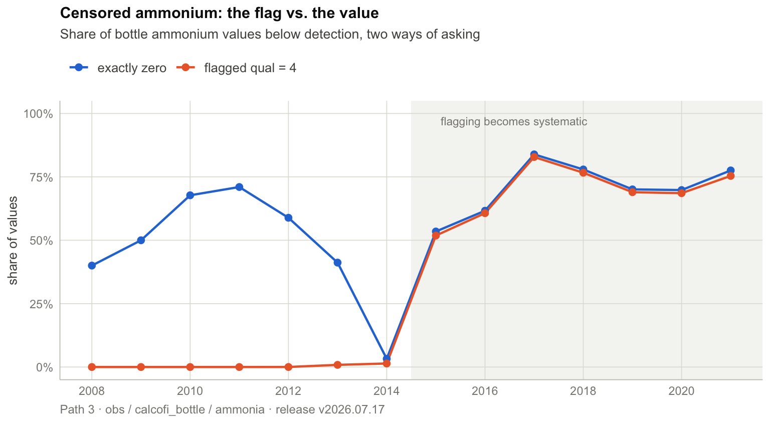
1. **Ammonium is a left-censored variable, and the censoring flag is not usable as
a time series.** 57.8 % of bottle ammonium values are *exactly* `0`, meaning
"below detection limit". But the flag that says so (`measurement_qual = 4`) is
essentially **unused before 2013** and applied to **69–84 % of values after
2015** — while the exact-zero fraction was *already* 40–71 % back in 2008–2012.
Filtering on the flag therefore removes ~0 % of the early record and ~75 % of the
late record, manufacturing a trend out of a change in laboratory bookkeeping.
The only censoring test that is consistent across the whole record is
`measurement_value == 0`.
2. **The 1.5 GB supplemental path yields *fewer* distinct measurements than the
thinned release, not more.** `obs_ctd_full`'s 134,597 `btl_ammonium` rows
collapse to **67,566** unique (occupation, depth) values — a **1.992×**
inflation, because each bottle value is written onto both the down- *and*
up-cast of every station occupation. Against the bottle table's 90,489 genuinely
distinct values, the big file is the *sparser* source, and it has lost the
quality flags. Its one real advantage is reach: it runs to **2025-04**, four
years past where the bottle series stops.
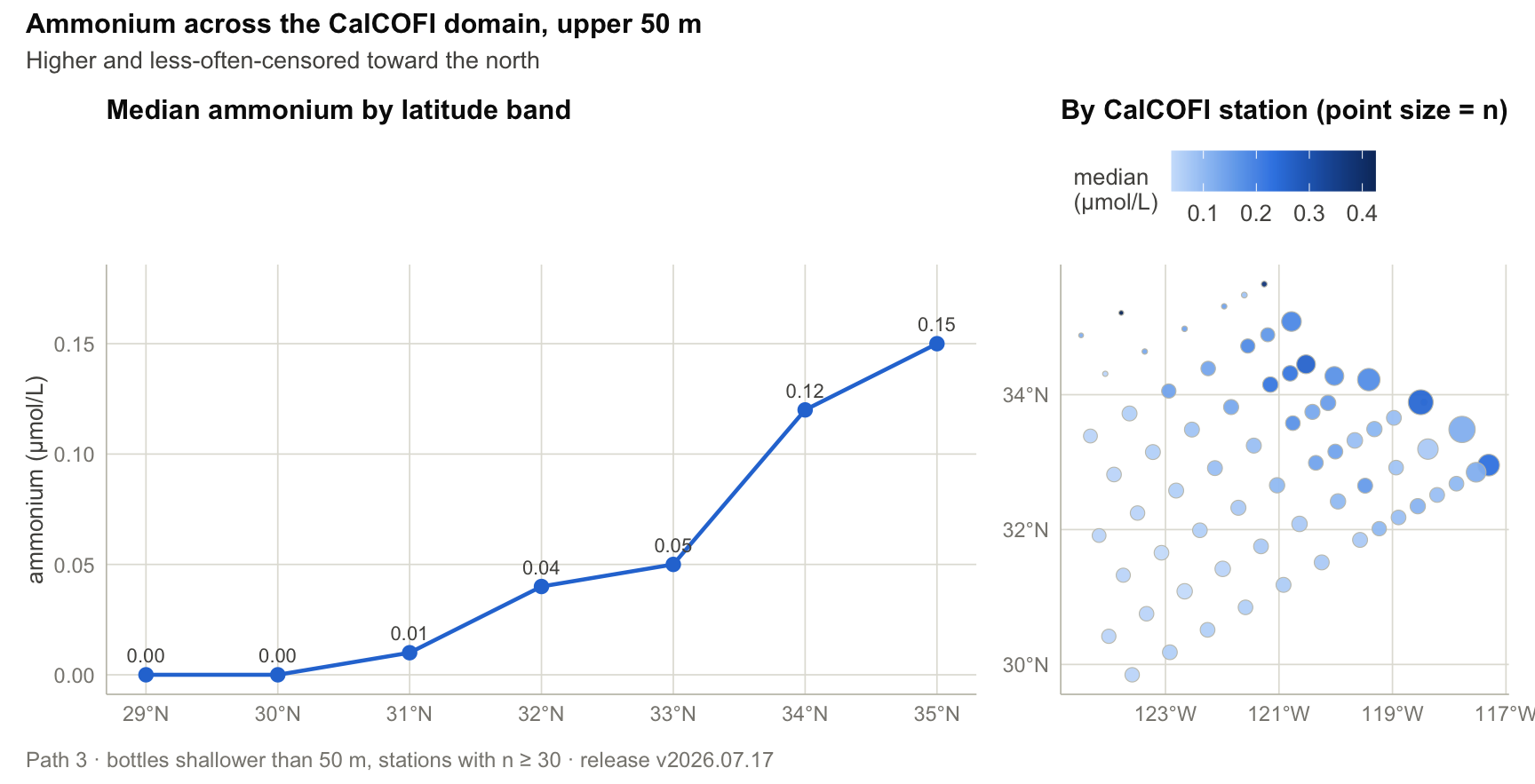
3. **The signal itself is clean and physically sensible once censoring is handled.**
Ammonium is a shallow, regenerated-nutrient feature: median 0.04–0.05 µmol/L in
the upper 50 m falling to ~0 below 100 m, with the censored (exactly-zero)
fraction rising from 34 % to 76 % over the same span; and a monotonic
south→north increase (median 0.00 → 0.15 µmol/L, 29°N → 35°N) tracking the
productivity gradient.
::: {.callout-tip title="Recommendation"}
For ammonium **over 2008–2021, use path 3** — `cc_get_db()` → `obs` filtered to
`dataset_key = 'calcofi_bottle'`, `measurement_type = 'ammonia'`. It is the only
path carrying the detection-limit flags, and it is one row per bottle. Reach for
path 4 **only** to extend past 2021, and then deduplicate cast direction first.
Neither NetCDF product is a usable ammonium source today; fixing path 2 is a
one-line change in the publish notebook (see [Open items](#open-items)).
:::
## Setup
```{r}
#| label: setup
#| message: false
#| warning: false
librarian::shelf(
  DBI, duckdb, dplyr, tidyr, ggplot2, glue, ncdf4, readr, scales,
  knitr, tibble, stringr, patchwork, sessioninfo, here, quiet = TRUE)
here <- here::here

# cc_release_version() / cc_release_partitions(): the repo's sanctioned way to
# resolve a release and enumerate a hive-partitioned table's objects. Reused
# rather than re-implemented so this notebook cannot drift from the publish step
# (and so the glob-404 workaround lives in exactly one place).
source(here("libs/publish_netcdf.R"))

RELEASE <- "v2026.07.17"
PQ      <- cc_release_parquet(RELEASE)
CACHE   <- here("data/cache"); dir.create(CACHE, recursive = TRUE, showWarnings = FALSE)

NC_URL   <- glue("https://storage.calcofi.io/calcofi-files-public/netcdf/ctd-cast/{RELEASE}/ctd-cast.nc")
NCF_URL  <- glue("https://storage.calcofi.io/calcofi-files-public/netcdf/ctd-cast_full/{RELEASE}/ctd-cast_full.nc")
NC_PATH  <- file.path(CACHE, "ctd-cast.nc")
NCF_PATH <- file.path(CACHE, "ctd-cast_full.nc")

cat(glue("release : {RELEASE}
          parquet : {PQ}
          cache   : {CACHE}\n"))
```
```{r}
#| label: palette
# Sequential encoding uses one hue light->dark; categorical series take fixed
# slots in a fixed order (never cycled), so a colour always means the same thing
# across figures. Palette validated for CVD separation and contrast on white.
CC_BLUE   <- "#2a78d6"   # categorical slot 1 / sequential hue
CC_ORANGE <- "#eb6834"   # slot 2
CC_AQUA   <- "#1baf7a"   # slot 3
CC_SEQ    <- c("#cde2fb", "#9ec5f4", "#6da7ec", "#3987e5", "#256abf", "#184f95", "#0d366b")
INK       <- "#0b0b0b"; INK2 <- "#52514e"; MUTED <- "#898781"
GRID      <- "#e1e0d9"; AXIS <- "#c3c2b7"

theme_cc <- function(base_size = 11) {
  theme_minimal(base_size = base_size) +
    theme(
      plot.title      = element_text(colour = INK,   face = "bold", size = rel(1.05)),
      plot.subtitle   = element_text(colour = INK2,  size = rel(0.92)),
      plot.caption    = element_text(colour = MUTED, size = rel(0.82), hjust = 0),
      axis.title      = element_text(colour = INK2,  size = rel(0.90)),
      axis.text       = element_text(colour = MUTED),
      panel.grid.major = element_line(colour = GRID, linewidth = 0.3),
      panel.grid.minor = element_blank(),
      axis.line        = element_line(colour = AXIS, linewidth = 0.3),
      strip.text       = element_text(colour = INK, face = "bold", size = rel(0.90)),
      legend.title     = element_text(colour = INK2, size = rel(0.88)),
      legend.text      = element_text(colour = INK2, size = rel(0.88)),
      legend.position  = "top", legend.justification = "left")
}
theme_set(theme_cc())

# cache a large remote file; skip the download when the local copy already
# matches the server's Content-Length (so re-renders are free)
cache_download <- function(url, path) {
  remote <- suppressWarnings(as.numeric(
    sub(".*[Cc]ontent-[Ll]ength:\\s*(\\d+).*", "\\1",
        paste(system(glue("curl -sI '{url}'"), intern = TRUE), collapse = " "))))
  if (file.exists(path) && isTRUE(file.size(path) == remote)) {
    cat(glue("cached: {basename(path)} ({round(file.size(path)/1048576,1)} MB)\n")); return(invisible(path))
  }
  cat(glue("downloading {basename(path)} ({round(remote/1048576,1)} MB) ...\n"))
  utils::download.file(url, path, mode = "wb", quiet = TRUE)
  invisible(path)
}
```
```{r}
#| label: connect
con <- dbConnect(duckdb())
for (s in c("INSTALL httpfs", "LOAD httpfs", "SET memory_limit='8GB'",
            "SET enable_progress_bar=false")) try(dbExecute(con, s), silent = TRUE)
q <- function(sql, ...) dbGetQuery(con, glue(sql, ..., .envir = parent.frame()))
```
## What "ammonium" is called, and where it lives
Before reading any product, ask the registry. `metadata/measurement_type.csv` is
the canonical vocabulary, and it already tells us that ammonium exists under
**three distinct names owned by two different datasets** — which is the root of
the whole comparison below.
```{r}
#| label: registry
read_csv(here("metadata/measurement_type.csv"), show_col_types = FALSE) |>
  filter(str_detect(measurement_type, "ammon")) |>
  select(measurement_type, description, units, is_canonical,
         source_column = `_source_column`, source_dataset = `_source_datasets`) |>
  kable()
```
`is_canonical` is the load-bearing column. The thinned CTD product keeps only
canonical sensors, and **`btl_ammonium` is not one** — so path 1 is already ruled
out before we open the file. The two bottle series *are* canonical, which is why
path 3 works.
## Path 1 — thinned CF NetCDF (`ctd-cast.nc`, 55 MB)
```{r}
#| label: nc-thin
cache_download(NC_URL, NC_PATH)
nc <- nc_open(NC_PATH)

thin_vars <- names(nc$var)
tibble(
  item  = c("profiles (casts)", "obs (depth levels)", "variables", "ammonium variables"),
  value = c(nc$dim[["profile"]]$len, nc$dim[["obs"]]$len, length(thin_vars),
            sum(grepl("ammon", thin_vars, ignore.case = TRUE))) |> as.character()) |>
  kable()
cat("variables:\n"); cat(strwrap(paste(sort(thin_vars), collapse = ", "), 78), sep = "\n")
nc_close(nc)
```
**Verdict: path 1 cannot answer the question.** There is no ammonium variable —
by design, as the registry predicted. This file is the right choice for
temperature/salinity/oxygen structure and the wrong one for nutrients.
## Path 2 — full-resolution CF NetCDF (`ctd-cast_full.nc`, 1.5 GB)
The companion file is advertised as a superset: every depth scan, and both cast
directions. It is reasonable to expect the sensor list to be a superset too.
```{r}
#| label: nc-full
cache_download(NCF_URL, NCF_PATH)
ncf <- nc_open(NCF_PATH)

full_vars <- names(ncf$var)
tibble(
  item  = c("profiles (casts)", "obs (depth levels)", "variables", "ammonium variables"),
  value = c(ncf$dim[["profile"]]$len, ncf$dim[["obs"]]$len, length(full_vars),
            sum(grepl("ammon", full_vars, ignore.case = TRUE))) |> as.character()) |>
  kable()
cat("variables:\n"); cat(strwrap(paste(sort(full_vars), collapse = ", "), 78), sep = "\n")
```
It is **not** a superset in the variable dimension. Here is why — and it is worth
stating precisely, because it is a fixable defect rather than a modelling choice.
`publish_ctd-cast_to-netcdf.qmd` derives the variable list from a **single
partition**:
```r
full_types <- dbGetQuery(con, glue(
  "SELECT DISTINCT measurement_type FROM read_parquet('{parts[1]}') ORDER BY 1"))$measurement_type
```
`parts[1]` is the alphabetically-first cruise, **1998-02-31JD**. Bottle nutrients
were not folded into the CTD cast files until 2008, so that cruise carries 32 of
the table's measurement types — and every type introduced later is silently
dropped from the published file.
```{r}
#| label: nc-full-diag
# the union across ALL partitions vs. what partition 1 alone would declare.
# Scanning measurement_type across 96 partitions costs ~95 s over the network,
# so cache the roll-up.
parts    <- cc_release_partitions("obs_ctd_full", RELEASE)
UNION_CSV <- file.path(CACHE, "ctd_full_type_union.csv")
if (!file.exists(UNION_CSV)) {
  urls <- paste0("'", parts, "'", collapse = ", ")
  dbExecute(con, glue("
    COPY (SELECT measurement_type, count(*) AS n_rows, count(DISTINCT cruise_key) AS n_cruises
          FROM read_parquet([{urls}], hive_partitioning = true)
          GROUP BY 1)
    TO '{UNION_CSV}' (HEADER)"))
}
type_union <- read_csv(UNION_CSV, show_col_types = FALSE)
p1_types   <- q("SELECT DISTINCT measurement_type FROM read_parquet('{p1}')",
                p1 = parts[1])$measurement_type

tibble(
  item = c(glue("measurement types in partition 1 ({basename(dirname(parts[1]))})"),
           glue("measurement types across all {length(parts)} partitions"),
           "types the published file therefore omits",
           "sensor variables actually in ctd-cast_full.nc"),
  value = as.character(c(
    length(p1_types), nrow(type_union),
    nrow(type_union) - length(intersect(type_union$measurement_type, p1_types)),
    length(setdiff(full_vars, c("profile_id","cruise_key","grid_key","time",
                                "latitude","longitude","rowSize","depth")))))) |>
  kable()
type_union |>
  filter(!measurement_type %in% p1_types) |>
  arrange(desc(n_rows)) |>
  select(measurement_type, n_rows, n_cruises) |>
  kable(caption = "Measurement types present in obs_ctd_full but absent from the published full NetCDF")
```
```{r}
#| label: nc-full-close
nc_close(ncf)
```
**Verdict: path 2 cannot answer the question either** — not because ammonium is
out of scope, but because of the single-partition type inference. Fixing it means
taking the union of types across partitions (the pass-1 loop already visits every
one).
::: {.callout-note title="What path 2 *does* demonstrate, for the record"}
Had the variable been declared, the read would be straightforward — a CF
contiguous ragged array expands to tidy rows with `rowSize` alone, no join:
```r
rs  <- ncvar_get(ncf, "rowSize")            # levels per profile
pix <- rep.int(seq_along(rs), rs)           # obs -> profile index
tibble(
  profile_id = ncvar_get(ncf, "profile_id")[pix],
  time       = as.POSIXct(ncvar_get(ncf, "time")[pix], origin = "1970-01-01", tz = "UTC"),
  latitude   = ncvar_get(ncf, "latitude")[pix],
  depth      = ncvar_get(ncf, "depth"),
  ammonium   = ncvar_get(ncf, "btl_ammonium")) |>
  filter(!is.na(ammonium))
```
That is the whole advantage of the DSG encoding: profile-level coordinates are
stored once and broadcast by index, so a 1.5 GB file needs no cross-referencing
to become a tidy frame.
:::
## Path 3 — release Parquet, thinned (`cc_get_db()`)
The `calcofi4r` entry point. `cc_get_db()` registers the release's Parquet as
remote DuckDB views; the default excludes supplemental tables.
```{r}
#| label: calcofi4r-thin
#| message: false
library(calcofi4r)

# NOTE: point cache_dir at this repo and set supplemental = TRUE up front. The
# local cache file is keyed on VERSION ONLY, so a plain cc_get_db() followed by
# cc_get_db(supplemental = TRUE) silently returns the cached 16-table connection
# with no obs_ctd_full. Opening it once, with supplemental, avoids the trap.
cc <- cc_get_db(version = RELEASE, supplemental = TRUE,
                cache_dir = file.path(CACHE, "calcofi4r"))
tbls <- sort(DBI::dbListTables(cc))
cat(glue("tables ({length(tbls)}): "), strwrap(paste(tbls, collapse = ", "), 74), sep = "\n")
```
First, confirm the thinned `obs` slice for the CTD dataset — the database-side
counterpart of path 1, and it agrees exactly:
```{r}
#| label: obs-ctd-types
DBI::dbGetQuery(cc, "
  SELECT count(DISTINCT measurement_type) AS ctd_sensor_types,
         count(DISTINCT measurement_type) FILTER (
           WHERE measurement_type ILIKE '%ammon%')  AS ammonium_types
  FROM obs WHERE dataset_key = 'calcofi_ctd-cast'") |> kable()
```
Now the slice that *does* carry ammonium — from `calcofi_bottle`. This is the
series the rest of the analysis uses.
```{r}
#| label: bottle-ammonia
amm <- DBI::dbGetQuery(cc, "
  SELECT sample_key, cruise_key, grid_key, latitude, longitude, datetime,
         depth_min_m AS depth_m, measurement_value AS ammonium, measurement_qual AS qual
  FROM obs
  WHERE dataset_key = 'calcofi_bottle' AND measurement_type = 'ammonia'") |>
  as_tibble() |>
  mutate(year = as.integer(format(datetime, "%Y")),
         is_bdl_flag = !is.na(qual) & qual == "4.0",
         is_zero     = ammonium == 0)

tibble(
  item = c("values", "distinct bottles", "temporal range", "depth range (m)",
           "value range (µmol/L)", "smallest positive value",
           "flagged below-detection (qual = 4)", "exactly zero", "exactly zero, unflagged"),
  value = c(
    format(nrow(amm), big.mark = ","),
    format(n_distinct(amm$sample_key), big.mark = ","),
    paste(format(min(amm$datetime), "%Y-%m-%d"), "to", format(max(amm$datetime), "%Y-%m-%d")),
    paste(min(amm$depth_m), "to", max(amm$depth_m)),
    paste(min(amm$ammonium), "to", max(amm$ammonium)),
    min(amm$ammonium[amm$ammonium > 0]),
    glue("{format(sum(amm$is_bdl_flag), big.mark=',')} ({round(100*mean(amm$is_bdl_flag),1)}%)"),
    glue("{format(sum(amm$is_zero), big.mark=',')} ({round(100*mean(amm$is_zero),1)}%)"),
    format(sum(amm$is_zero & !amm$is_bdl_flag), big.mark = ","))) |>
  kable()
```
Two things jump out. Every flagged value is *exactly* zero — so the flag means
"zeroed", per the CalCOFI convention where quality code **4 = "value zeroed due
to value below detection limit"**. And the smallest positive value in the whole
record is `0.01`, the reporting resolution — so zero is not a measurement, it is a
censoring marker.
```{r}
#| label: qual-crosstab
amm |>
  mutate(flag = if_else(is_bdl_flag, "qual = 4 (BDL)", "unflagged")) |>
  summarise(n = n(), exactly_zero = sum(is_zero),
            median = median(ammonium), max = max(ammonium), .by = flag) |>
  arrange(flag) |> kable()
```
But there are **24,579 unflagged exact zeros** — censored values that carry no
flag. That discrepancy is not random; it is chronological, and it is the subject
of the next section.
## Path 4 — release Parquet, supplemental (`obs_ctd_full`)
The supplemental table is 96 cruise partitions of full-resolution scans. Two
practical constraints shape how it must be read:
- A `read_parquet('.../obs_ctd_full/**/*.parquet')` glob **404s over HTTPS** —
expanding a glob needs a directory listing and object storage has none. Hence
`cc_release_partitions()`, which enumerates objects through the XML listing API.
- Filtering `measurement_type` across all 96 partitions takes **~95 s** over the
network. So extract once, cache to Parquet, and analyse locally.
```{r}
#| label: ctd-full-extract
AMM_PQ <- file.path(CACHE, "ctd_full_ammonium.parquet")
if (!file.exists(AMM_PQ)) {
  parts <- cc_release_partitions("obs_ctd_full", RELEASE)
  urls  <- paste0("'", parts, "'", collapse = ", ")
  dbExecute(con, glue("
    COPY (SELECT sample_key, cruise_key, grid_key, latitude, longitude, datetime,
                 depth_min_m, measurement_type, measurement_value, measurement_qual
          FROM read_parquet([{urls}], hive_partitioning = true)
          WHERE measurement_type = 'btl_ammonium')
    TO '{AMM_PQ}' (FORMAT parquet)"))
}

fullamm <- q("SELECT * FROM '{AMM_PQ}'") |>
  as_tibble() |>
  # sample_key is 'calcofi_ctd-cast:cast:<occupation><d|u>' — the trailing letter
  # is the cast DIRECTION, so the occupation is the key minus that letter.
  mutate(cast_dir   = str_extract(sample_key, "[du]$"),
         occupation = str_remove(sample_key, "[du]$"),
         year       = as.integer(format(datetime, "%Y")),
         is_zero    = measurement_value == 0)

tibble(
  item = c("rows", "distinct casts", "cruises", "temporal range",
           "value range (µmol/L)", "rows with a quality flag",
           "exactly zero", "distinct (occupation, depth) pairs", "row inflation"),
  value = c(
    format(nrow(fullamm), big.mark = ","),
    format(n_distinct(fullamm$sample_key), big.mark = ","),
    n_distinct(fullamm$cruise_key),
    paste(format(min(fullamm$datetime), "%Y-%m-%d"), "to", format(max(fullamm$datetime), "%Y-%m-%d")),
    paste(min(fullamm$measurement_value), "to", max(fullamm$measurement_value)),
    sum(!is.na(fullamm$measurement_qual)),
    glue("{format(sum(fullamm$is_zero), big.mark=',')} ({round(100*mean(fullamm$is_zero),1)}%)"),
    format(n_distinct(paste(fullamm$occupation, fullamm$depth_min_m)), big.mark = ","),
    round(nrow(fullamm) / n_distinct(paste(fullamm$occupation, fullamm$depth_min_m)), 3))) |>
  kable()
```
Two defects and one genuine gain:
```{r}
#| label: ctd-full-dir
fullamm |>
  summarise(rows = n(), casts = n_distinct(sample_key), .by = cast_dir) |>
  arrange(cast_dir) |> kable(caption = "Each bottle value appears on both cast directions")
```
- **Quality flags are gone** — `measurement_qual` is `NULL` for all 134,597 rows,
so the below-detection information that path 3 preserves does not survive here.
- **Every value is duplicated** across the down- and up-cast of each occupation
(1.992×). Aggregating without deduplicating double-weights every sample.
- **But it reaches four years further.** The bottle series ends 2021-05-13; this
one runs to 2025-04-18.
```{r}
#| label: path-compare
dedup <- fullamm |> distinct(occupation, depth_min_m, .keep_all = TRUE)

tibble(
  metric = c("distinct ammonium values", "temporal end", "below-detection flags",
             "grain", "bytes to read"),
  `path 3 — obs (thinned)` = c(
    format(nrow(amm), big.mark = ","), format(max(amm$datetime), "%Y-%m-%d"),
    "present (27,689 flagged)", "one row per bottle", "~2 MB (one Parquet slice)"),
  `path 4 — obs_ctd_full` = c(
    format(nrow(dedup), big.mark = ","), format(max(fullamm$datetime), "%Y-%m-%d"),
    "absent (all NULL)", "one row per cast-direction × depth", "~1.4 GB across 96 partitions")) |>
  kable()
```
**The thinned path holds more distinct ammonium values than the supplemental one**
— 90,489 against 67,566 — while being three orders of magnitude cheaper to read
and retaining the flags. "Full resolution" is a statement about CTD *scans*, not
about bottle nutrients.
## Ranges over time — and why the flag is unusable as a series {#over-time}
This is the finding that most changes an answer. Compare, per year, the share of
values **flagged** below-detection against the share that are **exactly zero**.
If the flag were applied consistently the two lines would coincide.
```{r}
#| label: fig-censoring
#| fig-width: 8
#| fig-height: 4.4
#| fig-cap: "The below-detection flag reflects laboratory bookkeeping, not ocean chemistry: it is essentially unused before 2013 while exact zeros already run 40–71%, then converges after 2015. Filtering on the flag would remove ~0% of the early record and ~75% of the late record."
by_year <- amm |>
  summarise(n = n(), pct_flagged = 100 * mean(is_bdl_flag),
            pct_zero = 100 * mean(is_zero), .by = year) |>
  arrange(year)

cens <- by_year |>
  select(year, `exactly zero` = pct_zero, `flagged qual = 4` = pct_flagged) |>
  pivot_longer(-year, names_to = "series", values_to = "pct")

ggplot(cens, aes(year, pct, colour = series)) +
  annotate("rect", xmin = 2014.5, xmax = Inf, ymin = -Inf, ymax = Inf,
           fill = GRID, alpha = 0.35) +
  annotate("text", x = 2015.1, y = 97, hjust = 0, size = 3, colour = MUTED,
           label = "flagging becomes systematic") +
  geom_line(linewidth = 0.8) +
  geom_point(size = 2.1) +
  scale_colour_manual(values = c("exactly zero" = CC_BLUE, "flagged qual = 4" = CC_ORANGE),
                      name = NULL) +
  scale_x_continuous(breaks = seq(2008, 2021, 2)) +
  scale_y_continuous(labels = label_percent(scale = 1), limits = c(0, 100)) +
  labs(title = "Censored ammonium: the flag vs. the value",
       subtitle = "Share of bottle ammonium values below detection, two ways of asking",
       x = NULL, y = "share of values",
       caption = "Path 3 · obs / calcofi_bottle / ammonia · release v2026.07.17") +
  theme(legend.position = "top")
```
```{r}
#| label: tbl-censoring
by_year |>
  transmute(year, n = format(n, big.mark = ","),
            `% flagged BDL` = round(pct_flagged, 1),
            `% exactly zero` = round(pct_zero, 1),
            `unflagged zeros` = round(pct_zero - pct_flagged, 1)) |>
  kable(caption = "The gap column is censored data with no flag — large before 2014, ~1 point after 2015")
```
Read the gap column top to bottom: 40 points of unflagged censoring in 2008,
71 in 2011, then ~1 point from 2015 on. **2014 is a third regime** — only 3.2 % of
that year's values are zero at all, against 41 % in 2013 and 53 % in 2015. That
discontinuity is not explained by the flag and is flagged below as an open
question.
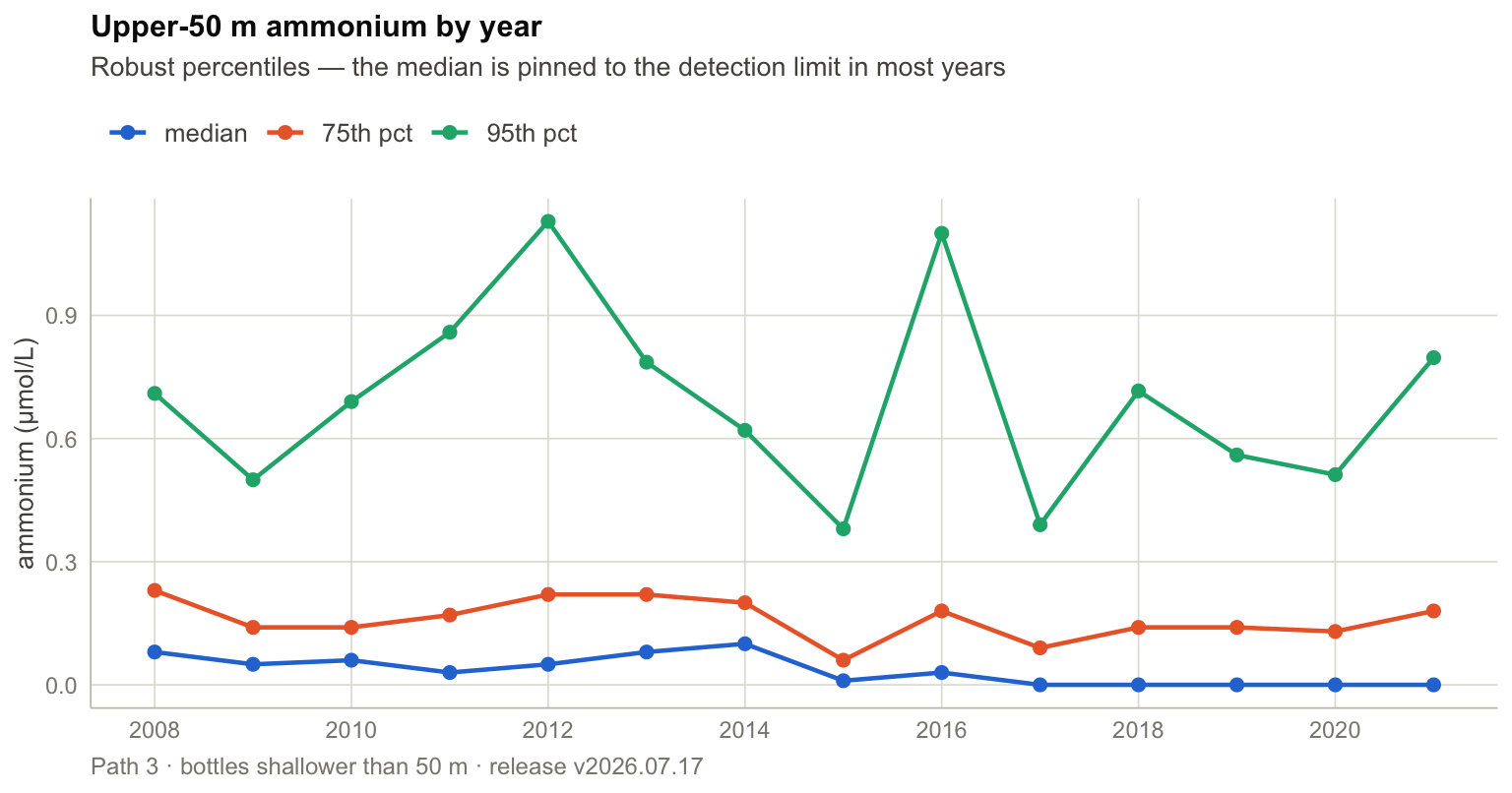
Now the actual ranges over time, computed the way a censored variable requires —
order statistics and a censored fraction, never a mean:
```{r}
#| label: fig-time-range
#| fig-width: 8
#| fig-height: 4.2
#| fig-cap: "Ammonium ranges by year in the upper 50 m, where the signal lives. Percentiles are robust to the censoring; the median sits at or near the detection limit in most years, so the upper percentiles carry the interannual signal."
upper <- amm |> filter(depth_m <= 50)

yr_rng <- upper |>
  summarise(n = n(), p50 = median(ammonium), p75 = quantile(ammonium, 0.75),
            p95 = quantile(ammonium, 0.95), .by = year) |>
  arrange(year)

yr_rng |>
  pivot_longer(c(p50, p75, p95), names_to = "stat", values_to = "value") |>
  # explicit factor levels: otherwise the legend orders alphabetically and puts
  # "95th pct" between "75th pct" and "median"
  mutate(stat = factor(c(p50 = "median", p75 = "75th pct", p95 = "95th pct")[stat],
                       levels = c("median", "75th pct", "95th pct"))) |>
  ggplot(aes(year, value, colour = stat)) +
  geom_line(linewidth = 0.8) + geom_point(size = 2) +
  scale_colour_manual(values = c("median" = CC_BLUE, "75th pct" = CC_ORANGE,
                                 "95th pct" = CC_AQUA), name = NULL) +
  scale_x_continuous(breaks = seq(2008, 2021, 2)) +
  labs(title = "Upper-50 m ammonium by year",
       subtitle = "Robust percentiles — the median is pinned to the detection limit in most years",
       x = NULL, y = "ammonium (µmol/L)",
       caption = "Path 3 · bottles shallower than 50 m · release v2026.07.17") +
  theme(legend.position = "top")
```
```{r}
#| label: tbl-time-range
yr_rng |>
  transmute(year, n = format(n, big.mark = ","),
            median = round(p50, 3), `75th pct` = round(p75, 3), `95th pct` = round(p95, 2)) |>
  kable(caption = "Upper-50 m ammonium percentiles by year (µmol/L)")
```
## Ranges over depth {#over-depth}
Ammonium is regenerated in and just below the euphotic zone and consumed
elsewhere, so depth is where the strongest structure should be — and is.
```{r}
#| label: fig-depth
#| fig-width: 9
#| fig-height: 4.4
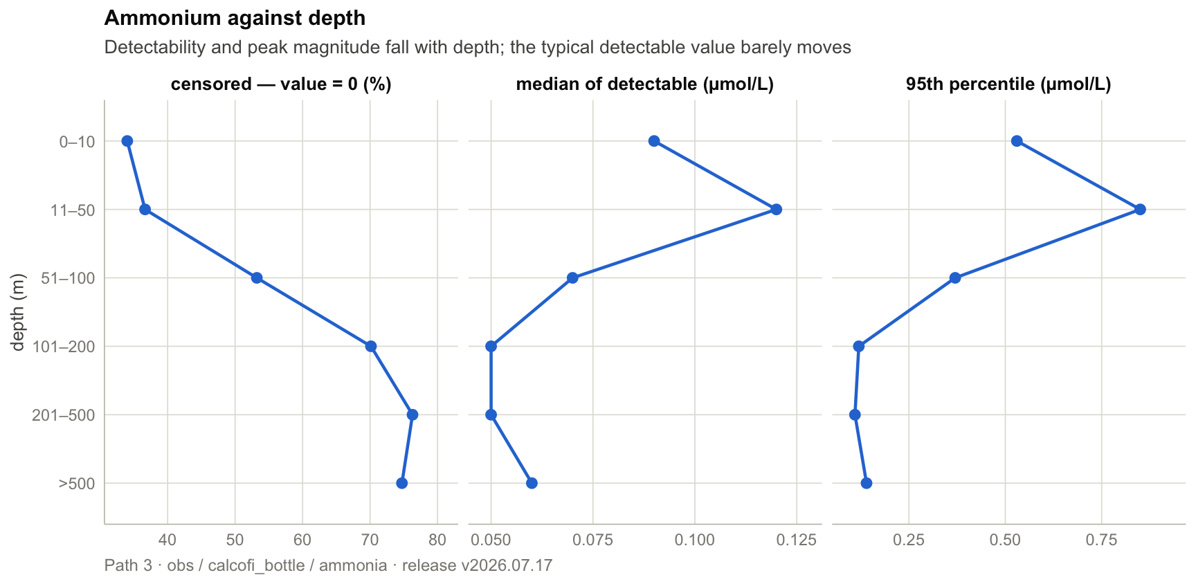
#| fig-cap: "Three views of the same depth transition, each on its own scale. What changes with depth is not the typical detectable concentration (centre, nearly flat at 0.05–0.12 µmol/L) but how *often* ammonium is detectable at all (left, 34% → 76% censored) and how high it peaks (right, a 7-fold fall in the 95th percentile)."
depth_bins <- c(0, 10, 50, 100, 200, 500, Inf)
depth_labs <- c("0–10", "11–50", "51–100", "101–200", "201–500", ">500")

by_depth <- amm |>
  mutate(bin = cut(depth_m, depth_bins, labels = depth_labs, include.lowest = TRUE)) |>
  summarise(n = n(),
            pct_zero = 100 * mean(is_zero), pct_flag = 100 * mean(is_bdl_flag),
            p50 = median(ammonium), p75 = quantile(ammonium, 0.75),
            p95 = quantile(ammonium, 0.95), max = max(ammonium),
            p50_pos = median(ammonium[ammonium > 0]), .by = bin) |>
  arrange(bin)

# Small multiples with free x rather than three series on one axis: the three
# quantities span an order of magnitude, so a shared scale flattens the two
# smaller ones into a vertical line. Facet strips name each measure, so no
# legend (and no colour) is needed to tell them apart.
by_depth |>
  select(bin,
         `censored — value = 0 (%)`        = pct_zero,
         `median of detectable (µmol/L)`   = p50_pos,
         `95th percentile (µmol/L)`        = p95) |>
  pivot_longer(-bin, names_to = "measure", values_to = "value") |>
  mutate(measure = factor(measure, levels = c(
    "censored — value = 0 (%)", "median of detectable (µmol/L)",
    "95th percentile (µmol/L)"))) |>
  ggplot(aes(value, bin, group = 1)) +
  geom_path(linewidth = 0.8, colour = CC_BLUE) +
  geom_point(size = 2.3, colour = CC_BLUE) +
  scale_y_discrete(limits = rev(depth_labs)) +
  scale_x_continuous(expand = expansion(mult = c(0.08, 0.16))) +
  facet_wrap(~measure, nrow = 1, scales = "free_x") +
  labs(title = "Ammonium against depth",
       subtitle = "Detectability and peak magnitude fall with depth; the typical detectable value barely moves",
       x = NULL, y = "depth (m)",
       caption = "Path 3 · obs / calcofi_bottle / ammonia · release v2026.07.17")
```
```{r}
#| label: tbl-depth
by_depth |>
  transmute(`depth (m)` = bin, n = format(n, big.mark = ","),
            `% zero` = round(pct_zero, 1), `% flagged` = round(pct_flag, 1),
            median = round(p50, 3), `median of positives` = round(p50_pos, 3),
            `75th pct` = round(p75, 3), `95th pct` = round(p95, 3), max = round(max, 2)) |>
  kable(caption = "Ammonium by depth stratum (µmol/L)")
```
The pooled median is `0` below 50 m — an artefact of censoring, not a
measurement, and the reason the *median of detectable values* is reported beside
it. Separating the two turns a vague "ammonium declines with depth" into a
sharper and more testable statement:
- **Detectability** collapses: 34 % of upper-10 m values are censored against
76 % at 201–500 m.
- **Peak magnitude** collapses with it: the 95th percentile falls 7-fold, from
0.85 µmol/L at 11–50 m to 0.11–0.14 µmol/L below 200 m.
- **The typical detectable value barely moves** — median of positives 0.09, 0.12,
0.07, 0.05, 0.05, 0.06 µmol/L from surface to bottom.
So depth does not scale ammonium down smoothly; it makes ammonium *rarer and less
peaky* while leaving the concentration of the detectable minority nearly
unchanged. That is consistent with ammonium as a locally-regenerated,
rapidly-consumed species — patches of it occur where remineralization is active,
and those patches are common and intense in the euphotic zone and sporadic below
it. A pooled mean would have collapsed all three of these into one downward
slope, and a pooled median would have shown zero.
## Ranges over space {#over-space}
Restricted to the upper 50 m, so the depth gradient above does not leak into the
spatial one.
```{r}
#| label: fig-space
#| fig-width: 9
#| fig-height: 4.6
#| fig-cap: "A monotonic south-to-north increase in upper-50 m ammonium (left) mirrored by a fall in the censored fraction from 60% to 13% — consistent with the productivity gradient across the CalCOFI domain. Right: per-station medians, sequential single-hue ramp."
by_lat <- upper |>
  mutate(lat_band = floor(latitude)) |>
  summarise(n = n(), pct_zero = 100 * mean(is_zero),
            p50 = median(ammonium), p50_pos = median(ammonium[ammonium > 0]),
            p95 = quantile(ammonium, 0.95), .by = lat_band) |>
  filter(n > 200) |> arrange(lat_band)

p_lat <- by_lat |>
  ggplot(aes(lat_band, p50)) +
  geom_line(linewidth = 0.8, colour = CC_BLUE) +
  geom_point(size = 2.4, colour = CC_BLUE) +
  geom_text(aes(label = sprintf("%.2f", p50)), vjust = -0.9, size = 2.9, colour = INK2) +
  scale_x_continuous(breaks = by_lat$lat_band, labels = paste0(by_lat$lat_band, "°N")) +
  expand_limits(y = max(by_lat$p50) * 1.18) +
  labs(title = "Median ammonium by latitude band",
       x = NULL, y = "ammonium (µmol/L)")

by_station <- upper |>
  summarise(n = n(), lat = median(latitude), lon = median(longitude),
            p50_pos = median(ammonium[ammonium > 0]), .by = grid_key) |>
  filter(n >= 30)

p_map <- by_station |>
  # shape 21 (fill + hairline stroke) so the palest sequential steps stay
  # visible against the white surface instead of dissolving into it
  ggplot(aes(lon, lat, fill = p50_pos, size = n)) +
  geom_point(shape = 21, colour = AXIS, stroke = 0.3, alpha = 0.95) +
  scale_fill_gradientn(colours = CC_SEQ, name = "median\n(µmol/L)") +
  scale_size_area(max_size = 5, guide = "none") +
  scale_x_continuous(labels = \(x) paste0(abs(x), "°W")) +
  scale_y_continuous(labels = \(y) paste0(y, "°N")) +
  coord_quickmap() +
  labs(title = "By CalCOFI station (point size = n)", x = NULL, y = NULL)

(p_lat | p_map) +
  patchwork::plot_annotation(
    title = "Ammonium across the CalCOFI domain, upper 50 m",
    subtitle = "Higher and less-often-censored toward the north",
    caption = "Path 3 · bottles shallower than 50 m, stations with n ≥ 30 · release v2026.07.17",
    theme = theme_cc())
```
```{r}
#| label: tbl-space
by_lat |>
  transmute(`latitude band` = paste0(lat_band, "°N"), n = format(n, big.mark = ","),
            `% zero` = round(pct_zero, 1), median = round(p50, 3),
            `median of positives` = round(p50_pos, 3), `95th pct` = round(p95, 2)) |>
  kable(caption = "Upper-50 m ammonium by 1° latitude band (µmol/L)")
```
The censored fraction and the concentration move in opposite directions across
the same gradient, which is the signature of a real signal rather than a sampling
artefact: were this driven by detection limits alone, both would move together.
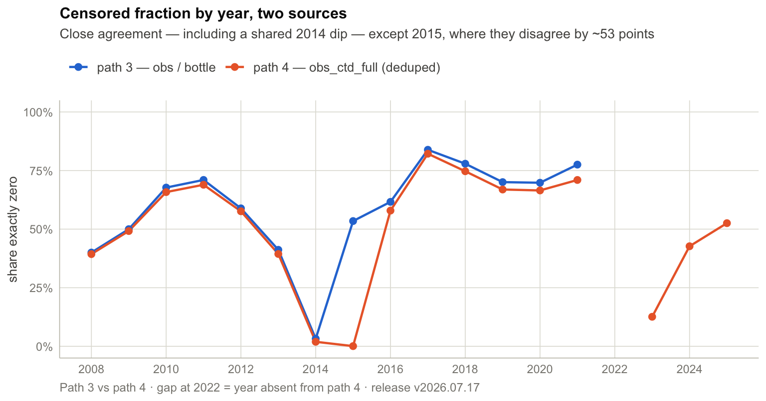
## Cross-checking path 3 against path 4
Do the two sources agree where they overlap? Compare annual medians from the
bottle table against the deduplicated CTD-embedded series.
```{r}
#| label: fig-cross
#| fig-width: 8
#| fig-height: 4.2
#| fig-cap: "The two sources track each other closely across the overlap — including a shared 2014 anomaly where both drop to ~2-3% censored — and disagree in exactly one year, 2015 (53% vs ~0%). The supplemental series extends to 2025 but skips 2022 entirely (the line is broken there rather than interpolated) and is thin in 2023."
cross <- bind_rows(
  amm   |> summarise(pct_zero = 100 * mean(is_zero), p50_pos = median(ammonium[ammonium > 0]),
                     n = n(), .by = year) |> mutate(src = "path 3 — obs / bottle"),
  dedup |> mutate(is_zero = measurement_value == 0) |>
           summarise(pct_zero = 100 * mean(is_zero),
                     p50_pos = median(measurement_value[measurement_value > 0]),
                     n = n(), .by = year) |> mutate(src = "path 4 — obs_ctd_full (deduped)")) |>
  # complete the year grid per source so a missing year (2022 in path 4) becomes
  # an explicit NA and geom_line breaks there instead of drawing a segment
  # across the gap, which would imply data that does not exist
  complete(src, year = full_seq(year, 1))

ggplot(cross, aes(year, pct_zero, colour = src)) +
  geom_line(linewidth = 0.8) + geom_point(size = 2.1) +
  scale_colour_manual(values = c("path 3 — obs / bottle" = CC_BLUE,
                                 "path 4 — obs_ctd_full (deduped)" = CC_ORANGE), name = NULL) +
  scale_x_continuous(breaks = seq(2008, 2025, 2)) +
  scale_y_continuous(labels = label_percent(scale = 1), limits = c(0, 100)) +
  labs(title = "Censored fraction by year, two sources",
       subtitle = "Close agreement — including a shared 2014 dip — except 2015, where they disagree by ~53 points",
       x = NULL, y = "share exactly zero",
       caption = "Path 3 vs path 4 · gap at 2022 = year absent from path 4 · release v2026.07.17")
```
```{r}
#| label: tbl-cross
cross |>
  select(year, src, pct_zero) |>
  pivot_wider(names_from = src, values_from = pct_zero) |>
  arrange(year) |>
  mutate(across(-year, \(x) round(x, 1)),
         gap = round(`path 4 — obs_ctd_full (deduped)` - `path 3 — obs / bottle`, 1)) |>
  kable(caption = "% exactly zero by year and source; NA = year absent from that source (2022 from path 4, 2023-25 from path 3)")
```
Two distinct things happen here, and they are worth separating:
- **2014 is a shared anomaly.** Both sources drop to ~2–3 % censored, against
41 % in 2013 and 53 % in 2015. Because *both* show it, it is a real feature of
that year's reporting rather than a discrepancy between products — that year's
values were apparently not zeroed. Any trend fitted through 2014 will be
distorted regardless of which path is used.
- **2015 is a genuine disagreement.** The bottle table reports 53 % censored; the
CTD-embedded copy ~0 %. Both cannot describe the same water. It is *not* a
pre- versus post-QC distinction — the bottle table's own pre-QC `r_ammonium`
also reports 53 % — so one of the two products carries the wrong ammonium
column for that year. This one needs a provenance answer before 2015 is used
from path 4.
## Caveats and open items {#open-items}
**Statistical.** Ammonium here is **left-censored at the detection limit**, with
58 % of values censored overall and up to 84 % in some years. Everything above
uses censored fractions plus order statistics, and reports the median of positive
values alongside the pooled median. A publication-grade treatment should go
further — Kaplan–Meier or maximum-likelihood estimation for censored data (e.g.
the `NADA` approach) — and should *not* substitute zero, half the detection
limit, or the mean of the raw column. Because the censoring *rate* itself changes
through the record, interannual comparisons of any central-tendency statistic are
confounded regardless of estimator.
**Coverage.** The bottle ammonium series begins 2008-01-07, not at the start of
the CalCOFI record; there is no pre-2008 ammonium in this release. Path 4 skips
2022 entirely and has only 758 rows for 2023.
**Open items for the pipeline**, in priority order:
| # | Item | Where |
|---|---|---|
| 1 | `full_types` is inferred from `parts[1]`, so any measurement type absent from cruise 1998-02-31JD is silently dropped from `ctd-cast_full.nc`. Take the union across partitions (the pass-1 loop already visits every one). | `publish_ctd-cast_to-netcdf.qmd` |
| 2 | `measurement_qual` is `NULL` for all `btl_ammonium` in `obs_ctd_full`, losing the below-detection flag that `obs` retains. | ctd-cast ingest |
| 3 | Bottle values are written onto both cast directions in `obs_ctd_full`, so bottle-derived types are 1.99× duplicated. Either restrict them to one direction or document the required dedup. | ctd-cast ingest |
| 4 | **2015** censoring disagrees between the bottle table (53 %) and the CTD-embedded copy (~0 %); not a QC-stage difference, since pre-QC `r_ammonium` also reads 53 %. Which column did each product take? | data question |
| 4b | **2014** shows ~3 % censoring in *both* sources against 41 % in 2013 and 53 % in 2015 — that year's values appear not to have been zeroed. Confirm and document. | data question |
| 5 | 24,579 unflagged exact zeros in 2008–2013 are censored values without `qual = 4`. Backfill the flag, or document that `value == 0` is the portable test. | bottle ingest |
| 6 | `cc_get_db()`'s local cache is keyed on version only, so a later `supplemental = TRUE` call silently returns a connection without `obs_ctd_full`. | `calcofi4r::cc_get_db()` |
```{r}
#| label: cleanup
DBI::dbDisconnect(cc, shutdown = TRUE)
dbDisconnect(con, shutdown = TRUE)
```
## Session
```{r}
#| label: session
sessioninfo::session_info(pkgs = c("calcofi4r", "duckdb", "ncdf4", "ggplot2"))$packages |>
  as_tibble() |> select(package, loadedversion, source) |> kable()
```