---
title: "CTD derived hydrographic products: a first stab"
subtitle: "Spice, mixed-layer depth, chlorophyll-a maximum, integrated chlorophyll-a, averaged sigma-theta and relative geostrophic velocity, on one cruise"
author: "CalCOFI"
date: today
format:
html:
toc: true
toc-depth: 3
code-fold: true
code-tools: true
df-print: kable
fig-align: center
editor_options:
chunk_output_type: console
---
## Why
Rasmus Swalethorp asked, at the CTD-on-EDI meeting (2026-09-16) and by email (2026-09-22), for
**derived hydrographic products** beside the measured CTD series. These are values computed from the
profiles that say "how much upwelling might be going on on our grid at that specific time of the
cruise, how much productivity might there be". He wants them in the transect plotter and the
Explorer within about two months, for the public interest in the developing El Niño. The plan is in
[CalCOFI/workflows#98](https://github.com/CalCOFI/workflows/issues/98), with one issue per product
(#99–#103).
This is a **prototype**, not an ingest. It has no `calcofi:` targets block, so it is not part of the
pipeline or a release. It reads one cruise's **full-resolution** CTD casts (`obs_ctd_full`, 1 m bins)
from the published release. It applies the rules now in `calcofi4db` (≥ 4.16.0: `ctd_spice()`,
`ctd_mld()`, `ctd_chl_max()`, `ctd_integrate()`, `ctd_sigma_theta_ave()`, `ctd_geostrophic()`),
then draws each product so Rasmus can judge the defaults before they become a dataset.
::: {.callout-note title="Defaults that need Rasmus's confirmation"}
- **MLD**: reference **10 m**, Δσθ = **0.03 kg m⁻³** (de Boyer Montégut et al. 2004), drawn beside
Δσθ = 0.125 kg m⁻³ (Levitus 1982) and |ΔT| = 0.2 °C.
- **Chlorophyll-a maximum**: a **5 m running median** before taking the maximum.
- **Integrated chlorophyll-a**: surface to **200 m**, trapezoidal.
- **Geostrophic velocity**: reference **500 dbar**, carrying the deepest density down for shallower
casts, as in his script; those pairs are flagged. Stations **closer than 10 km** to the previous
one are skipped (the extra inshore stations, e.g. SCCOOS 90.27.7 beside 90.28), because the shear
scales as `1 / dx`.
- **Cast**: the **down** cast (`…d`) of each station; the release also carries the up cast (`…u`).
:::
```{r}
#| label: setup
librarian::shelf(
  calcofi4db, calcofi4r, DBI, dplyr, tidyr, ggplot2, glue, maps, quiet = T)
stopifnot(packageVersion("calcofi4db") >= "4.16.0")

ver    <- "v2026.09.11"   # the promoted release on 2026-09-23 (latest.txt)
cruise <- "2025-04-3322"  # the latest cruise with bottle data (preliminary_with_bottle)
lines  <- c(90, 80)

cat_ <- cc_catalog(ver)
con  <- dbConnect(duckdb::duckdb())
invisible(dbExecute(con, "INSTALL httpfs; LOAD httpfs"))

# obs_ctd_full is hive-partitioned by cruise_key: read only this cruise's object
src_full <- cc_release_sources(cat_, "obs_ctd_full")
url_full <- grep(glue("cruise_key={cruise}/"), src_full$urls, fixed = TRUE, value = TRUE)
stopifnot(length(url_full) == 1)
invisible(dbExecute(con, paste0(
  "CREATE VIEW sample AS SELECT * FROM ", cc_read_parquet_sql(cc_release_sources(cat_, "sample")))))
```
## Read one cruise
```{r}
#| label: read
types <- c(
  "pressure", "temperature_ave", "salinity_ave_corr", "sigma_theta_1", "sigma_theta_2",
  "est_chlorophyll_a_sta_corr")

long <- dbGetQuery(con, glue("
  SELECT f.sample_key, s.site_key, s.data_stage, f.latitude, f.longitude,
         f.depth_min_m AS depth_m, f.measurement_type AS type,
         f.measurement_value AS val, f.measurement_qual AS qual
  FROM read_parquet('{url_full}') f
  JOIN sample s USING (sample_key)
  WHERE f.measurement_type IN ({paste0(\"'\", types, \"'\", collapse = ', ')})
    AND right(f.sample_key, 1) = 'd'"))

prof <- long |>
  pivot_wider(
    id_cols = c(sample_key, site_key, data_stage, latitude, longitude, depth_m),
    names_from = type, values_from = c(val, qual), values_fn = mean) |>
  rename_with(~ sub("^val_", "", .x)) |>
  mutate(
    line    = as.numeric(substr(site_key, 1, 5)),
    station = as.numeric(substr(site_key, 7, 11))) |>
  arrange(line, station, depth_m)

# every qual_* column the pivot produced, blank when the release carried no flag
for (tp in types) if (!paste0("qual_", tp) %in% names(prof)) prof[[paste0("qual_", tp)]] <- NA

# one row per cast: position varies along a cast (the ship drifts), so take its first fix
casts <- prof |>
  group_by(sample_key, site_key, line, station, data_stage) |>
  summarize(latitude = first(latitude), longitude = first(longitude), .groups = "drop")
cat(glue(
  "{cruise}: {nrow(casts)} down casts on {n_distinct(casts$line)} lines, ",
  "{nrow(prof)} 1 m bins, data_stage {paste(unique(casts$data_stage), collapse = ', ')}"), "\n")
cat(glue(
  "flagged values in this cruise's obs_ctd_full: ",
  "{sum(!is.na(long$qual) & sub('\\\\.0+$', '', long$qual) %in% c('8', '9'))}"), "\n")
```
## Per-sample products: averaged sigma-theta and spice
The averaged sigma-theta is the flag rule every CTD pair follows
([#99](https://github.com/CalCOFI/workflows/issues/99)). Spice is Rasmus's recipe
([#100](https://github.com/CalCOFI/workflows/issues/100)): TEOS-10 `gsw_spiciness0()` from the
sensor-pair averaged, corrected temperature and salinity, not sensor 1.
```{r}
#| label: per-sample
prof <- prof |>
  mutate(
    sigma_theta_ave = ctd_sigma_theta_ave(
      sigma_theta_1, sigma_theta_2, qual_sigma_theta_1, qual_sigma_theta_2),
    spice = ctd_spice(
      temperature_ave, salinity_ave_corr, pressure, longitude, latitude,
      qual_temperature_ave, qual_salinity_ave_corr))

# distance along the line from its nearshore-most station, drawn offshore on the left
haversine_km <- function(lat1, lon1, lat2, lon2) {
  p1 <- lat1 * pi / 180; p2 <- lat2 * pi / 180
  a  <- sin((p2 - p1) / 2)^2 + cos(p1) * cos(p2) * sin((lon2 - lon1) * pi / 360)^2
  2 * 6371 * atan2(sqrt(a), sqrt(1 - a))
}
casts <- casts |>
  group_by(line) |>
  mutate(dist_km = haversine_km(
    latitude[which.min(station)], longitude[which.min(station)], latitude, longitude)) |>
  ungroup()
prof <- left_join(prof, select(casts, sample_key, dist_km), by = "sample_key")

spice_rng <- range(prof$spice, na.rm = TRUE)
cat(glue("spice: {sprintf('%.2f', spice_rng[1])} to {sprintf('%.2f', spice_rng[2])} kg m^-3"), "\n")
```
```{r}
#| label: fig-spice
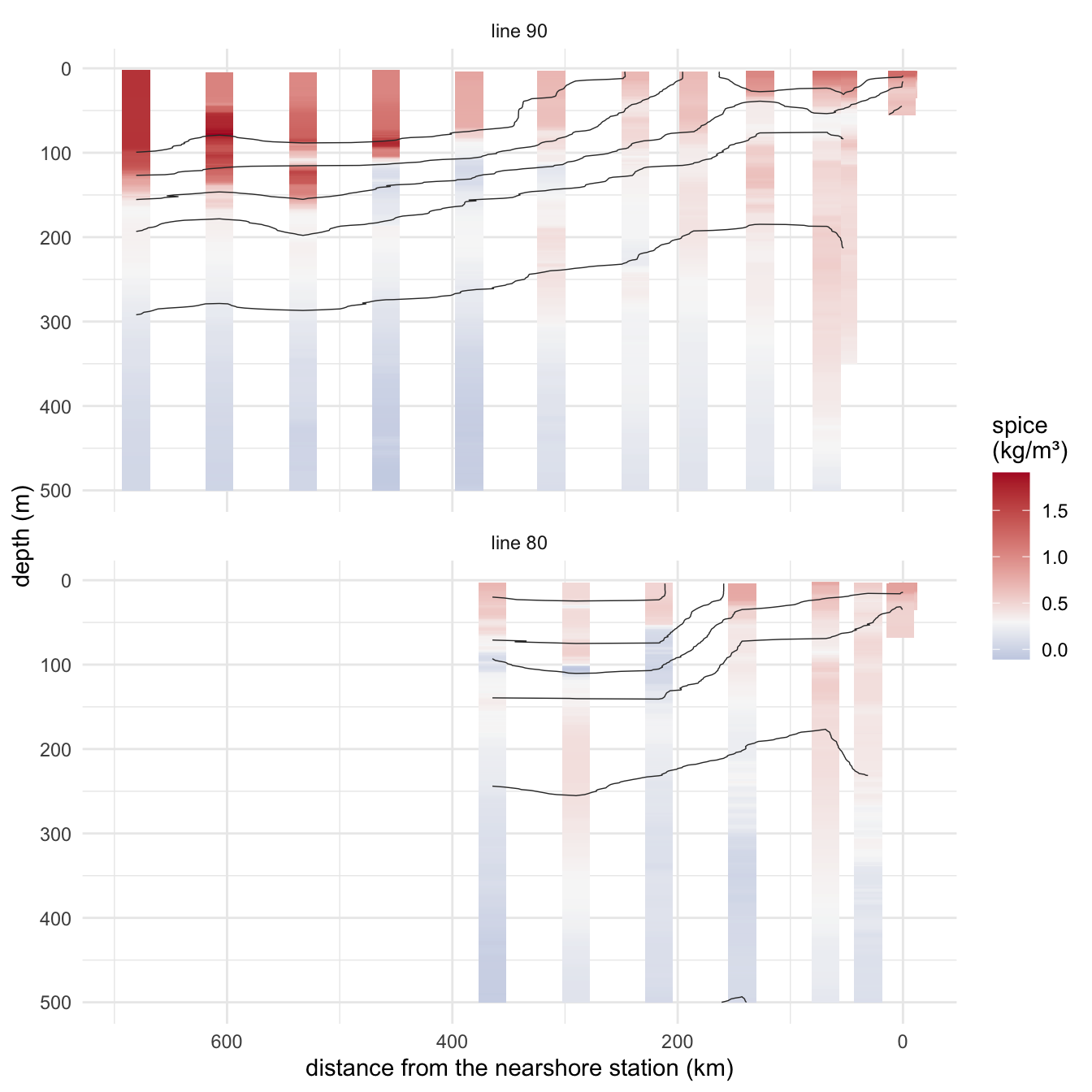
#| fig-cap: "Spice (spiciness at 0 dbar) on lines 90 and 80, 0–500 m. Red is spicy (warm, salty), blue minty (cool, fresh), centred on the section median. Offshore is on the left, as in the transect plotter. Contours are averaged sigma-theta."
#| fig-height: 7
sec <- prof |>
  filter(line %in% lines, depth_m <= 500) |>
  mutate(line = factor(glue("line {line}"), levels = glue("line {lines}")))

ggplot(sec, aes(dist_km, depth_m)) +
  geom_tile(aes(fill = spice), width = 25, height = 1) +
  geom_contour(aes(z = sigma_theta_ave), colour = "grey20", linewidth = 0.25,
               breaks = seq(23, 27.5, 0.5)) +
  scale_fill_gradient2(
    low = "#2166ac", mid = "#f7f7f7", high = "#b2182b",
    midpoint = median(sec$spice, na.rm = TRUE), name = "spice\n(kg/m³)") +
  scale_x_reverse() + scale_y_reverse() +
  facet_wrap(~line, ncol = 1) +
  labs(x = "distance from the nearshore station (km)", y = "depth (m)") +
  theme_minimal()
```
## Per-cast products: mixed-layer depth
MLD by three criteria, side by side ([#101](https://github.com/CalCOFI/workflows/issues/101)). The
temperature criterion needs no salinity, so it is the only one a `preliminary_without_bottle` cruise
could have.
```{r}
#| label: mld
mld <- prof |>
  group_by(sample_key) |>
  group_modify(~ bind_rows(
    ctd_mld(.x$depth_m, .x$sigma_theta_ave, criterion = "sigma_theta", threshold = 0.03) |>
      mutate(crit = "Δσθ 0.03 (default)"),
    ctd_mld(.x$depth_m, .x$sigma_theta_ave, criterion = "sigma_theta", threshold = 0.125) |>
      mutate(crit = "Δσθ 0.125"),
    ctd_mld(.x$depth_m, .x$temperature_ave, criterion = "temperature", threshold = 0.2,
            qual = .x$qual_temperature_ave) |>
      mutate(crit = "|ΔT| 0.2 °C"))) |>
  ungroup() |>
  left_join(casts, by = "sample_key")

mld_sum <- mld |>
  group_by(criterion = crit) |>
  summarize(
    casts = n(), ok = sum(status == "ok"),
    mixed_to_bottom = sum(status == "mixed_to_bottom"), no_reference = sum(status == "no_reference"),
    `median MLD (m)` = median(mld_m, na.rm = TRUE),
    `min (m)` = min(mld_m, na.rm = TRUE), `max (m)` = max(mld_m, na.rm = TRUE), .groups = "drop")
mld_sum
```
```{r}
#| label: fig-mld-map
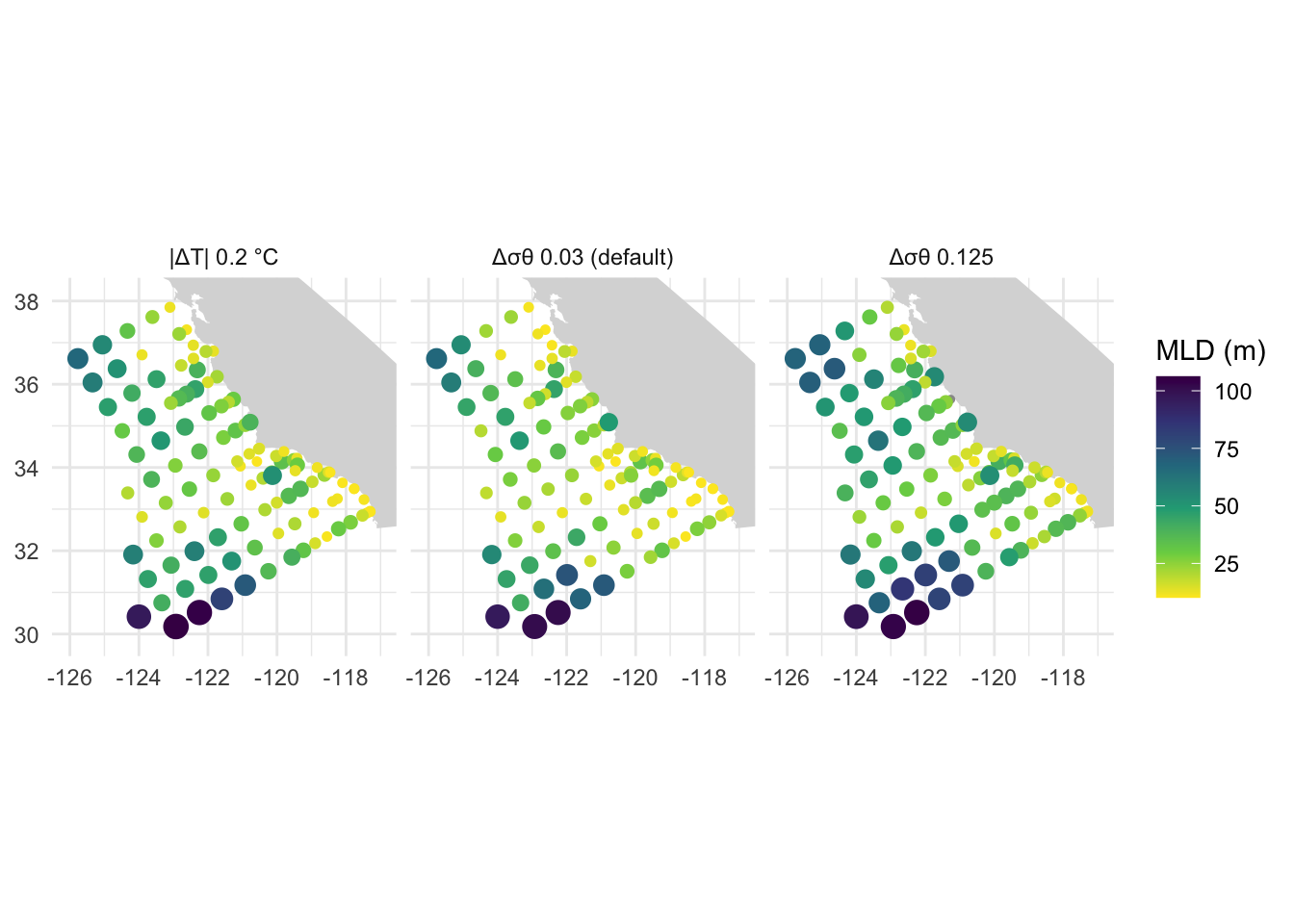
#| fig-cap: "Mixed-layer depth per down cast by each criterion. Larger points are deeper mixed layers; grey casts never crossed the threshold or lack the 10 m reference."
#| fig-height: 5
coast <- map_data("state", region = "california")
ggplot() +
  geom_polygon(data = coast, aes(long, lat, group = group), fill = "grey85") +
  geom_point(data = filter(mld, status != "ok"), aes(longitude, latitude), colour = "grey60", size = 1) +
  geom_point(data = filter(mld, status == "ok"),
             aes(longitude, latitude, colour = mld_m, size = mld_m)) +
  scale_colour_viridis_c(direction = -1, name = "MLD (m)") +
  scale_size_area(max_size = 4, guide = "none") +
  coord_quickmap(xlim = range(casts$longitude) + c(-0.3, 0.3),
                 ylim = range(casts$latitude) + c(-0.3, 0.3)) +
  facet_wrap(~crit) +
  labs(x = NULL, y = NULL) + theme_minimal()
```
## Per-cast products: chlorophyll-a maximum and integrated chlorophyll-a
From the bottle-fitted sensor estimate `est_chlorophyll_a_sta_corr`, the series Rasmus chose on
2026-09-09 ([#102](https://github.com/CalCOFI/workflows/issues/102)).
```{r}
#| label: chl
chl <- prof |>
  group_by(sample_key) |>
  group_modify(~ bind_cols(
    ctd_chl_max(.x$depth_m, .x$est_chlorophyll_a_sta_corr, .x$qual_est_chlorophyll_a_sta_corr),
    ctd_integrate(.x$depth_m, .x$est_chlorophyll_a_sta_corr, .x$qual_est_chlorophyll_a_sta_corr,
                  z_max = 200))) |>
  ungroup() |>
  left_join(casts, by = "sample_key")

chl |>
  summarize(
    casts = n(), `with chl` = sum(n > 0),
    `chl max depth, median (m)` = median(chl_max_depth_m, na.rm = TRUE),
    `chl max depth, range (m)` = paste(range(chl_max_depth_m, na.rm = TRUE), collapse = "–"),
    `integrated 0–200 m, median (mg/m²)` = round(median(integrated, na.rm = TRUE), 1),
    `integrated, range (mg/m²)` = paste(round(range(integrated, na.rm = TRUE), 1), collapse = "–"),
    `status ok` = sum(status == "ok"), shallow = sum(status == "shallow"),
    no_surface = sum(status == "no_surface"))
```
```{r}
#| label: fig-chl-map
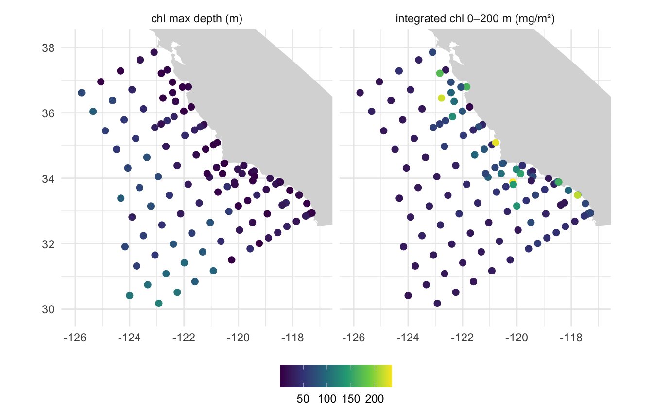
#| fig-cap: "Depth of the chlorophyll-a maximum (left) and chlorophyll-a integrated over 0–200 m (right), per down cast. The deep chlorophyll maximum deepens and the integral falls offshore, away from the upwelling."
#| fig-height: 4.5
chl_long <- bind_rows(
  transmute(chl, longitude, latitude, product = "chl max depth (m)", v = chl_max_depth_m),
  transmute(chl, longitude, latitude, product = "integrated chl 0–200 m (mg/m²)", v = integrated))
ggplot() +
  geom_polygon(data = coast, aes(long, lat, group = group), fill = "grey85") +
  geom_point(data = filter(chl_long, !is.na(v)), aes(longitude, latitude, colour = v), size = 2) +
  scale_colour_viridis_c(name = NULL) +
  coord_quickmap(xlim = range(casts$longitude) + c(-0.3, 0.3),
                 ylim = range(casts$latitude) + c(-0.3, 0.3)) +
  facet_wrap(~product) +
  labs(x = NULL, y = NULL) + theme_minimal() + theme(legend.position = "bottom")
```
## Per-station-pair product: relative geostrophic velocity
Rasmus's recipe ([#103](https://github.com/CalCOFI/workflows/issues/103)): dynamic height relative to
500 dbar, `v = Δ(dynamic height) / (f · dx)` between adjacent stations. Stations are ordered
nearshore → offshore, so **positive is equatorward** (90° to the left of the offshore direction, on
a line that runs west-south-west). It is relative flow, so there is **no anomaly view**.
```{r}
#| label: geo
geo <- lapply(lines, function(ln) {
  d <- prof |>
    filter(line == ln) |>
    transmute(
      station = site_key, station_order = station, latitude, longitude, dist_km,
      pressure, temperature = temperature_ave, salinity = salinity_ave_corr,
      q_temperature = qual_temperature_ave, q_salinity = qual_salinity_ave_corr)
  ctd_geostrophic(d, p_ref = 500, min_dx_km = 10) |> mutate(line = ln)
}) |> bind_rows()

geo_sum <- geo |>
  group_by(line) |>
  summarize(
    pairs = n_distinct(paste(station_1, station_2)),
    `shallow pairs` = n_distinct(paste(station_1, station_2)[shallow]),
    `max equatorward (m/s)` = round(max(velocity_m_s[!shallow]), 3),
    `max poleward (m/s)` = round(min(velocity_m_s[!shallow]), 3),
    `shallow pairs: max |v| (m/s)` = round(max(abs(velocity_m_s[shallow]), 0), 3), .groups = "drop")
geo_sum
```
```{r}
#| label: fig-geo
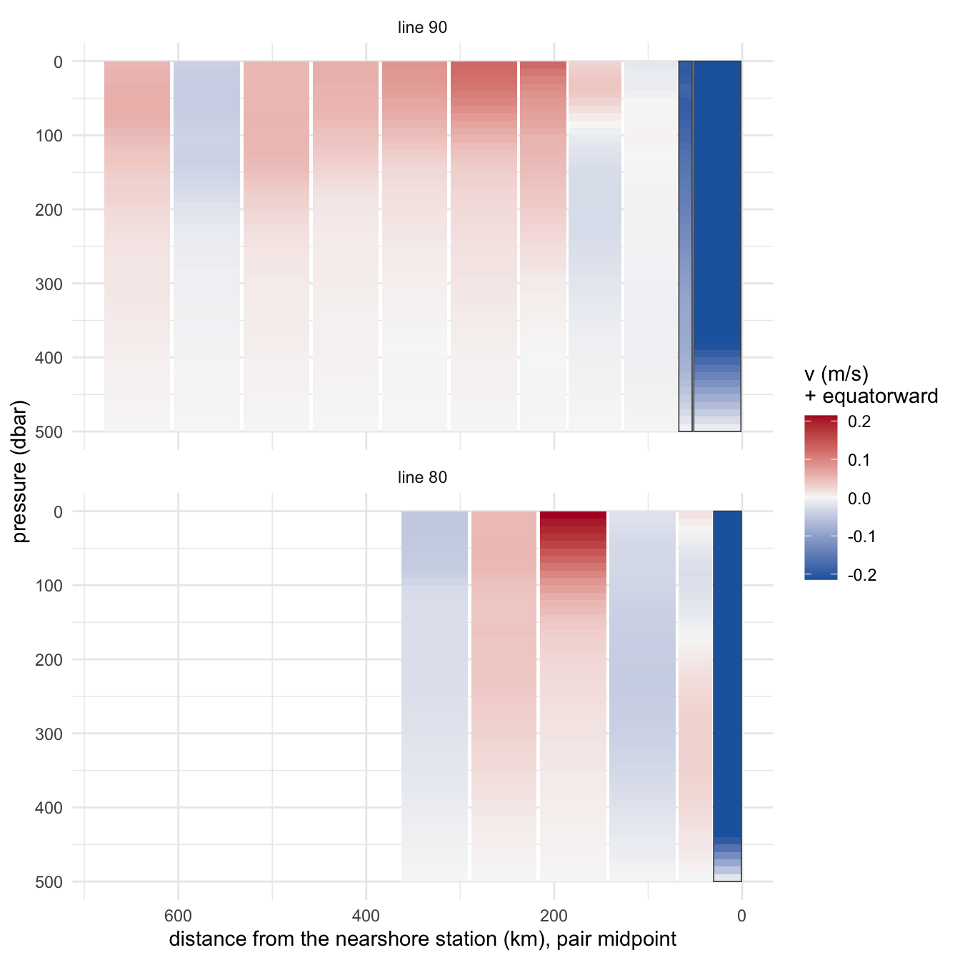
#| fig-cap: "Relative geostrophic velocity between adjacent stations on lines 90 and 80, referenced to 500 dbar, averaged to 10 dbar. Red is equatorward (the California Current), blue poleward (the California Undercurrent near the slope). Each column is a station pair at its midpoint. Outlined pairs include a cast shallower than 500 dbar; their reference is carried down, and the colour scale is set by the other pairs, so they saturate."
#| fig-height: 7
geo10 <- geo |>
  mutate(p10 = floor((pressure - 1) / 10) * 10 + 5) |>
  group_by(line, station_1, station_2, dist_mid_km, dx_km, shallow, p10) |>
  summarize(v = mean(velocity_m_s), .groups = "drop") |>
  mutate(line = factor(glue("line {line}"), levels = glue("line {lines}")))
# scale on the pairs that reach 500 dbar; a shelf pair's carried-down reference can saturate
lim <- max(abs(geo10$v[!geo10$shallow]))
ggplot(geo10, aes(dist_mid_km, p10)) +
  geom_tile(aes(fill = v, width = dx_km * 0.95), height = 10) +
  geom_tile(data = distinct(filter(geo10, shallow), line, dist_mid_km, dx_km),
            aes(x = dist_mid_km, y = 250, width = dx_km * 0.95), height = 500,
            fill = NA, colour = "grey30", linewidth = 0.3, inherit.aes = FALSE) +
  scale_fill_gradient2(
    low = "#2166ac", mid = "#f7f7f7", high = "#b2182b", midpoint = 0,
    limits = c(-lim, lim), oob = scales::squish, name = "v (m/s)\n+ equatorward") +
  scale_x_reverse() + scale_y_reverse() +
  facet_wrap(~line, ncol = 1) +
  labs(x = "distance from the nearshore station (km), pair midpoint", y = "pressure (dbar)") +
  theme_minimal()
```
## What this says about the defaults
```{r}
#| label: takeaways
mld_med <- setNames(mld_sum$`median MLD (m)`, mld_sum$criterion)
geo_ok  <- filter(geo, !shallow)
```
- **MLD:** the choice of criterion matters more than anything else here. On `r cruise` the median
MLD is `r round(mld_med[["Δσθ 0.03 (default)"]])` m by Δσθ 0.03,
`r round(mld_med[["Δσθ 0.125"]])` m by Δσθ 0.125 and `r round(mld_med[["|ΔT| 0.2 °C"]])` m by
|ΔT| 0.2 °C. 0.03 finds the most recent mixing, 0.125 the top of the seasonal pycnocline. Every
cast bracketed the 10 m reference, and only `r sum(mld$status == "mixed_to_bottom")` never crossed
a threshold. **Rasmus to choose.**
- **Spice:** it ranges from `r sprintf("%.2f", spice_rng[1])` to `r sprintf("%.2f", spice_rng[2])`
kg m⁻³ on this cruise. The spiciest water is the warm, salty offshore surface layer, while the deep
offshore water is minty (subarctic California Current water). Nearshore on line 90, the water at
100–300 m is spicier than offshore at the same depth, which is where the California Undercurrent
carries equatorial water north. That is the signal Rasmus expects an El Niño to strengthen; an
anomaly against the release climatology comes once spice is a released `measurement_type`.
- **Geostrophic velocity:** pairs that reach 500 dbar run
`r round(min(geo_ok$velocity_m_s), 2)` to `r round(max(geo_ok$velocity_m_s), 2)` m s⁻¹, the
O(0.1 m s⁻¹) expected for the California Current system. The **shelf pairs** (a cast shallower
than 500 dbar, reference carried down as in the recipe) reach
`r round(max(abs(geo$velocity_m_s[geo$shallow])), 2)` m s⁻¹, which is not credible. Referencing them to
the shallower cast's bottom (a "bottom-depth" or deepest-common-level reference) is the
alternative to put to Rasmus.
- **Chlorophyll-a:** the maximum sits at `r median(chl$chl_max_depth_m, na.rm = TRUE)` m (median),
deepening offshore. `r sum(chl$status == "shallow")` of `r nrow(chl)` casts end above 200 m, so
their integral stops at the bottom and says so (`status = shallow`).
```{r}
#| label: cleanup
dbDisconnect(con, shutdown = TRUE)
```