---
title: "Ingest CalCOFI Phytoplankton (Venrick)"
calcofi:
target_name: ingest_calcofi_phytoplankton
workflow_type: ingest
dependency:
- ingest_swfsc_ichthyo
output: data/parquet/calcofi_phytoplankton/manifest.json
provider: calcofi
dataset: phytoplankton
workflow_url: https://calcofi.io/workflows/ingest_calcofi_phytoplankton.html
questions_file: metadata/calcofi/phytoplankton/questions.csv
dataset_meta:
dataset_name: CalCOFI Phytoplankton (Venrick)
# display trio, read by the release `dataset` table and the
# consumer apps (calcofi4db >= 3.15.0) — see NEWS for why these
# left the apps' own hardcoded maps
dataset_name_short: Phytoplankton
category: Phytoplankton
color: "#0b7454"
# publishes the consolidated core. Region-pooled: sample rows carry
# sample_type = region_pool with a NULL grid_key, and obs carries no datetime.
tables_owned:
- {table: sample, shared: true, note: "core event dimension (region_pool grain, no grid_key)"}
- {table: obs, shared: true, note: "core occurrence headline (bio, cell abundance by taxon)"}
- {table: taxon, shared: true, note: "shared taxa reference"}
- {table: dataset_taxon, shared: true, note: "species_code -> taxon_key crosswalk"}
- {table: taxon_group, shared: true, note: "phytoplankton functional groups"}
- {table: region, note: "pooled-region reference; POLYGON geometry derived from the station membership declared in definitions.xlsx"}
- {table: measurement_type, shared: true}
erd:
color: "#b5e8b0"
editor_options:
chunk_output_type: console
---
## Overview
**Source**: EDI [`knb-lter-cce.254.4`](https://portal.edirepository.org/nis/mapbrowse?packageid=knb-lter-cce.254.4)
— *Temporal and spatial changes of the abundance and species composition of
phytoplankton in the California Current* (E. Venrick + CalCOFI + CCE-LTER,
1996-2022). Provider `calcofi`.
**Grain note**: samples are **pooled across stations into 4 regions** before
counting, so there is no per-station `site_key`. We model the native grain —
`phyto_sample` = one row per (cruise × region) — and link to the cruise registry
by year-month (`cruise_key`).
Each region carries a **polygon derived from the station membership the source
declares**, not a position we chose: `cc_station_regions()` gives every declared
station the water nearest to it and dissolves those cells by region, so the four
regions tile their pooled domain exactly — no overlap, no gaps, each one
connected. The point on `phyto_sample` is a representative point *inside* that
polygon, which is what replaced the provisional centroid (see Questions Q01).
## Setup
```{r}
#| label: setup
#| message: false
devtools::load_all(here::here("../calcofi4db"))
devtools::load_all(here::here("../calcofi4r"))
librarian::shelf(
  CalCOFI/calcofi4db, CalCOFI/calcofi4r,
  DBI, dplyr, DT, fs, glue, here, janitor, jsonlite, knitr, lubridate, purrr,
  readr, readxl, sf, stringr, tibble, tidyr, units, quiet = T)
options(readr.show_col_types = F); options(DT.options = list(scrollX = TRUE))
source(here("libs/ingest.R"))
source(here("libs/parse_phytoplankton.R"))
cc <- read_calcofi_meta(here("ingest_calcofi_phytoplankton.qmd"))
provider <- cc$provider; dataset <- cc$dataset; tables_owned <- cc$tables_owned
dir_label   <- glue("{provider}_{dataset}")
dir_parquet <- here(glue("data/parquet/{dir_label}"))
dir_stage <- cc_stage_path("parquet", dir_label, create = TRUE)
db_path     <- here(glue("data/wrangling/{dir_label}.duckdb"))
if (overwrite && file_exists(db_path)) file_delete(db_path)
dir_create(dirname(db_path)); con <- get_duckdb_con(db_path); load_duckdb_extension(con, "spatial")
meas_type_csv <- here("metadata/measurement_type.csv"); d_meas_type <- read_measurement_type(meas_type_csv)
```
## Download from EDI
```{r}
#| label: download
dir_dl <- here(glue("data/cache/{dir_label}")); dir_create(dir_dl)
edi_base <- "https://pasta.lternet.edu/package/data/eml/knb-lter-cce/254/4"
edi_ents <- c(
  abund_1996_2012 = "f2c2349b1b8f3f743913ddcf9b39339c",
  abund_2012_2018 = "d59e83016505f8a802df8519ca6eba06",
  abund_2019_2022 = "e683e945180ea0e5093aebe88f3d5c76",
  definitions     = "97d8f56bf41502f60ca6fdd5d5da8edc")
for (nm in names(edi_ents)) {
  f <- file.path(dir_dl, paste0(nm, ".xlsx"))
  if (overwrite_all || !file_exists(f)) download.file(paste0(edi_base, "/", edi_ents[[nm]]), f, quiet = TRUE)
}
cat(glue("Downloaded {length(edi_ents)} EDI entities to {dir_dl}"), "\n")
if (Sys.getenv("CALCOFI_SKIP_GCS") == "") {
  sync_to_gcs(local_dir = dir_dl, gcs_prefix = glue("archive/{provider}/{dataset}"),
              bucket = "calcofi-files-public", exclude = c(".DS_Store"))
} else cat("CALCOFI_SKIP_GCS set - skipping the upload (local verification run)\n")
```
## Parse + Clean
The per-year sheets are taxon × (cruise × region) cross-tabs with merged 2-row
headers; `parse_phyto_workbooks()` (in `libs/parse_phytoplankton.R`) flattens
them to long form. We then drop stray file-path cells and separate the
group-`SUM` rows (derivable from the taxa, excluded per Q03).
```{r}
#| label: parse
abund_files <- file.path(dir_dl, c("abund_1996_2012.xlsx","abund_2012_2018.xlsx","abund_2019_2022.xlsx"))
d_long <- parse_phyto_workbooks(abund_files) |> mutate(species_code = str_trim(species_code))
d_long <- d_long |> mutate(
  is_path = str_detect(species_code, "^[a-zA-Z]:\\\\|forweb"),
  is_sum  = str_detect(str_to_upper(species_code), "^SUM"),
  is_num  = str_detect(species_code, "^[0-9]+$"))
d_taxa_long <- d_long |> filter(is_num)
cat(glue("parsed {nrow(d_long)} rows: {sum(d_long$is_path)} path-junk dropped, ",
         "{sum(d_long$is_sum)} group-SUM excluded, {nrow(d_taxa_long)} taxon-level kept"), "\n")
```
## Build Region (polygons from the declared station membership)
The source tells us exactly which CalCOFI stations were pooled into each region
— `definitions.xlsx` sheet `Regions`, citing Hayward & Venrick 1998 — so read
that rather than inventing a position. Membership is all it gives; the geometry
is derived from it by `calcofi4db::cc_station_regions()` (workflows#76 Q01).
```{r}
#| label: region
# Read the membership verbatim from the source, so a provider correction lands
# by re-running rather than by editing a tribble in this notebook. Rows above
# the "Abbreviation" header are the citation, and the sheet has no column names.
reg_raw <- read_excel(file.path(dir_dl, "definitions.xlsx"), sheet = "Regions",
                      col_names = FALSE, .name_repair = "minimal") |>
  setNames(c("region_key", "description", "station_codes"))
hdr <- which(str_detect(reg_raw$region_key, regex("^abbreviation$", ignore_case = TRUE)))
stopifnot("`Regions` sheet must carry its Abbreviation header" = length(hdr) == 1)
reg_defs <- reg_raw |>
  slice((hdr + 1):n()) |>
  filter(!is.na(region_key), !is.na(station_codes)) |>
  mutate(across(everything(), str_squish))

# The sheet writes each station as a ROUNDED-line shorthand plus a station
# number: "87.40" is line 86.7 station 40, NOT line 87.4. Three encodings of one
# grid are in play -- this shorthand, `cc_grid`'s truncated integer (86), and the
# release `grid` table's decimal (86.7) -- and matching the wrong one is silent.
line_map <- c(`77` = 76.7, `80` = 80.0, `83` = 83.3,
              `87` = 86.7, `90` = 90.0, `93` = 93.3)
reg_sta <- reg_defs |>
  mutate(code = str_split(station_codes, ",")) |>
  select(region_key, code) |> unnest(code) |> mutate(code = str_trim(code)) |>
  mutate(line    = unname(line_map[str_extract(code, "^[0-9]+")]),
         station = as.numeric(str_extract(code, "[0-9]+$")))
stopifnot(
  "every station code parses to a known CalCOFI line" = !anyNA(reg_sta$line),
  "every station code carries a station number"       = !anyNA(reg_sta$station))

# Positions come from the +proj=calcofi transform, not a `grid` lookup: six of
# the 34 declared stations (83.41, 83.51, 90.37, 77.51, 80.51, 90.53) are
# intermediate inshore stations with no cell in the regularized grid, and a
# lookup drops them with no error. Three of the six are NE's -- the region
# closest to shore, where this dataset's gradient is steepest.
region_sf <- cc_station_regions(reg_sta, group = "region_key")

region <- reg_defs |>
  select(region_key, description, station_codes) |>
  inner_join(st_drop_geometry(region_sf), by = "region_key") |>
  mutate(geom_wkt = st_as_text(st_geometry(region_sf))[match(region_key, region_sf$region_key)]) |>
  select(region_key, description, latitude, longitude, n_stations, station_codes, geom_wkt)
stopifnot(
  "every declared region got geometry" = nrow(region) == nrow(reg_defs),
  "station membership is preserved"    = sum(region$n_stations) == nrow(reg_sta))

# CTAS rather than ALTER + UPDATE: mutating a table that carries a GEOMETRY
# column trips a DuckDB checkpoint bug (see CLAUDE.md).
dbWriteTable(con, "region_wkt", region, overwrite = TRUE)
dbExecute(con, "
  CREATE OR REPLACE TABLE region AS
  SELECT region_key, description, latitude, longitude, n_stations, station_codes,
         ST_GeomFromText(geom_wkt) AS geom
  FROM region_wkt")
dbExecute(con, "DROP TABLE region_wkt")
stopifnot(
  "every region is a single polygon" =
    dbGetQuery(con, "SELECT COUNT(*) FROM region
                     WHERE geom IS NULL OR ST_GeometryType(geom) <> 'POLYGON'")[[1]] == 0)
cat(glue("region: {nrow(region)} polygons over {nrow(reg_sta)} declared stations, ",
         "all placed by +proj=calcofi (Q01)"), "\n")
datatable(region |> select(-geom_wkt),
          caption = "Pooled regions: derived polygons + an interior representative point")
```
## Build Sample (cruise × region) + cruise_key match
```{r}
#| label: sample
# cruise registry (year-month -> cruise_key, unique months only)
load_prior_tables(con, parquet_dir = cc_stage_path("parquet", "swfsc_ichthyo"),
                  tables = c("cruise","ship","grid"), geom_tables = c("grid"), as_view = TRUE)
cr <- dbGetQuery(con, "SELECT cruise_key, date_ym FROM cruise") |>
  mutate(ym = format(as.Date(date_ym), "%Y%m"))
ck <- cr |> group_by(ym) |>
  summarize(cruise_key = if (n() == 1) cruise_key[1] else NA_character_, .groups = "drop")

phyto_sample <- d_taxa_long |>
  distinct(cruise_yymm, year, month, region_key = region) |>
  mutate(ym = sprintf("%04d%02d", year, month)) |>
  left_join(ck, by = "ym") |>
  left_join(region |> select(region_key, latitude, longitude), by = "region_key") |>
  arrange(year, month, region_key) |>
  transmute(
    phyto_sample_id = row_number(),
    cruise_yymm, cruise_key, year, month,
    season = recode(as.integer(month), `1`="winter",`2`="winter",`3`="spring",`4`="spring",
                    `5`="spring",`6`="summer",`7`="summer",`8`="summer",`9`="fall",
                    `10`="fall",`11`="fall",`12`="winter", .default = NA_character_),
    region_key, latitude, longitude)
dbWriteTable(con, "phyto_sample", phyto_sample, overwrite = TRUE)
add_point_geom(con, "phyto_sample", lon_col = "longitude", lat_col = "latitude")
cat(glue("phyto_sample {nrow(phyto_sample)} (4 regions x {n_distinct(phyto_sample$cruise_yymm)} cruises); ",
         "cruise_key matched {sum(!is.na(phyto_sample$cruise_key))}/{nrow(phyto_sample)} (Q06)"), "\n")
```
## Build Taxon (verbatim + WoRMS) + Measurement
```{r}
#| label: taxon-measurement
# WoRMS aphia_ids resolved + cached in metadata/.../taxon_worms.csv (Q05).
# `species` is the source's name, verbatim (and the name a consumer displays);
# `name_query` is what was looked up; `aphia_id` is the key. Rules (2026-09-28,
# B7 2026-10-01; libs/verify_phyto_aphia.R re-checks them against WoRMS):
# - a clear spelling slip is fixed in the query only (Rhisosolenia -> Rhizosolenia,
#   brightwelli -> brightwellii); the species keys its accepted WoRMS record
# - an unknown species of a named genus -- "sp. 1", "sp. a", "spp.", "uncertain
#   species", a size class, spores, a "complex", a "cf." determination, a species
#   WoRMS does not hold, and species of ONE genus counted together ("A + A. b") --
#   keys that genus. The genus is the ACCEPTED one: where WoRMS files the source's
#   species under another accepted genus the genus codes key that genus, so a
#   hierarchy rollup agrees with the species items ("Ceratium spp." keys Tripos,
#   as the Ceratium species do), while `species` keeps "Ceratium spp."
# - species of two genera counted together key the lowest common ancestor of the
#   two genera in WoRMS's classification (Dactyliosolen + Guinardia ->
#   Rhizosoleniaceae), never a class a family would do instead; Q09 asks the provider
# Calcidiscus leptoporus (worms:235923) and Rhabdosphaera clavigera (worms:235972)
# are accepted species the WoRMS name services never return; they are filled from
# their AphiaID records.
worms <- read_csv(here("metadata/calcofi/phytoplankton/taxon_worms.csv")) |>
  mutate(species_code = as.character(species_code))
phyto_taxon <- worms |>
  transmute(species_code, taxa, species,
            aphia_id = as.integer(aphia_id), scientific_name_accepted, rank, kingdom, phylum)
# codes present in the abundance data but absent from the Definitions sheet (Q05):
# add placeholder rows so phyto_measurement.species_code has a complete FK.
missing_codes <- setdiff(unique(d_taxa_long$species_code), phyto_taxon$species_code)
if (length(missing_codes) > 0)
  phyto_taxon <- bind_rows(phyto_taxon, tibble(
    species_code = missing_codes, taxa = "undefined (code not in source definitions; Q05)",
    species = NA_character_, aphia_id = NA_integer_, scientific_name_accepted = NA_character_,
    rank = NA_character_, kingdom = NA_character_, phylum = NA_character_))
dbWriteTable(con, "phyto_taxon", phyto_taxon, overwrite = TRUE)

phyto_meas_src <- d_taxa_long |>
  inner_join(phyto_sample |> select(phyto_sample_id, cruise_yymm, region_key),
             by = c("cruise_yymm", "region" = "region_key")) |>
  filter(!is.na(abundance)) |>
  transmute(phyto_sample_id, cruise_yymm, region_key = region, species_code,
            measurement_type = "phytoplankton_abundance", measurement_value = abundance)

# Duplicate (sample, species_code) rows (workflows#124, WS-1004X) ----
# Two row sets carry the same species code twice in one sample, so a summed
# abundance doubles (a presence count does not):
#  (1) cruises 0704, 1202, 1203 -- 1,496 codes x 4 regions each. 1202 and 1203 sit
#      in both the 1996-2012 and the 2012-2018 workbook (Q06), and the 2007 sheet
#      has two columns both labelled "CalCOFI 0704".
#  (2) species code 178 in 53 further samples (1902-2211): the same row twice.
# Decision (Ben, WS-1004X brief 2026-10-04): where the two rows hold the SAME value, drop the second
# -- the repeat adds nothing. Where they DIFFER, keep both on an explicit allowlist
# until the provider answers Q06: we cannot tell which row is right, and choosing one
# would be inventing a value. The allowlist is keyed by cruise x region x code (a
# phyto_sample_id is a row_number and moves when a cruise is added).
dup_differing <- read_csv(here("metadata/calcofi/phytoplankton/duplicate_pairs_differing.csv"),
                          col_types = cols(.default = "c")) |>
  select(cruise_yymm, region_key, species_code)
n_src_rows    <- nrow(phyto_meas_src)
phyto_measurement <- phyto_meas_src |>
  distinct(phyto_sample_id, species_code, measurement_value, .keep_all = TRUE) |>
  select(-cruise_yymm, -region_key) |>
  mutate(phyto_measurement_id = row_number(), .before = 1)
n_dup_dropped <- n_src_rows - nrow(phyto_measurement)

# uniqueness gate: (phyto_sample_id, species_code) is unique outside the allowlist,
# and the allowlist lists exactly the pairs still duplicated (an entry that no longer
# duplicates must be removed; a new duplicate must fail here, not reach append_obs()).
dup_left <- phyto_measurement |>
  count(phyto_sample_id, species_code) |> filter(n > 1) |>
  inner_join(phyto_sample |> select(phyto_sample_id, cruise_yymm, region_key),
             by = "phyto_sample_id")
stopifnot(
  "(phyto_sample_id, species_code) is not unique outside the Q06 allowlist -- a new duplicate pair" =
    nrow(anti_join(dup_left, dup_differing, by = c("cruise_yymm", "region_key", "species_code"))) == 0,
  "duplicate_pairs_differing.csv lists a pair that is no longer duplicated: remove it" =
    nrow(anti_join(dup_differing, dup_left, by = c("cruise_yymm", "region_key", "species_code"))) == 0,
  "the differing-value pairs left in place must stay the 290 measured at WS-1004X" =
    nrow(dup_left) == 290,
  "identical-value duplicate rows dropped must stay the 4,251 measured at WS-1004X (4,198 pairs + 53 code-178)" =
    n_dup_dropped == 4251)
cat(glue("duplicates: {n_dup_dropped} identical-value repeat rows dropped; ",
         "{nrow(dup_left)} differing pairs kept on the Q06 allowlist"), "\n")
dbWriteTable(con, "phyto_measurement", phyto_measurement, overwrite = TRUE)
cat(glue("phyto_taxon {nrow(phyto_taxon)} ({sum(!is.na(phyto_taxon$aphia_id))} WoRMS-matched); ",
         "phyto_measurement {nrow(phyto_measurement)}"), "\n")
# Codes that reach ONLY a class ----
# A code with no AphiaID in taxon_worms.csv and no ds_taxa_code row in
# metadata/taxon_override.csv falls through to the six ds_common_name rows there
# and keys the class (Bacillariophyceae, Dinophyceae, ...). That is right for the
# source's own unidentified classes ("indistinguished pennate diatoms", "pennate
# sp. 6"); it is wrong for a named taxon whose lookup failed. Until 2026-09-28, 53
# codes were that -- among them both Pseudo-nitzschia size classes, Calcidiscus
# leptoporus and Ditylum brightwellii -- so "Diatoms, not identified further"
# silently absorbed named taxa. A code that keys a class by its AphiaID (rank
# Class: code 77, whose lowest common ancestor IS the class) is the same finding.
# `taxa = "other"` rows are excluded: no class row reaches them; they resolve by
# code override or key dataset-locally (local_allow, below).
ovr_codes <- read_csv(here("metadata/taxon_override.csv"), show_col_types = FALSE) |>
  filter(dataset_key == "calcofi_phytoplankton", match_column == "ds_taxa_code") |>
  pull(match_value) |> as.character()
class_only <- phyto_taxon |>
  filter((is.na(aphia_id) & !species_code %in% ovr_codes) | rank %in% "Class",
         !is.na(species), taxa != "other") |>
  select(species_code, taxa, species)
# the allowlist: ONE code at a time, with the reason. Sixteen are the source's own
# unidentified classes; code 77 counts a named Mastogloia with an unidentified
# pennate, whose lowest common ancestor is the class. A named taxon that fails its
# lookup is not on this list, so it fails the render instead of vanishing into a class.
class_allow <- tibble::tribble(
  ~species_code, ~why,
  "603", "source's own unidentified class: indistinguished diatom species",
  "85",  "source's own unidentified class: pennate sp. 1",
  "243", "source's own unidentified class: pennate sp. 2",
  "318", "source's own unidentified class: pennate sp. 3",
  "401", "source's own unidentified class: pennate sp. 4",
  "508", "source's own unidentified class: pennate sp. 5",
  "512", "source's own unidentified class: pennate sp. 6",
  "608", "source's own unidentified class: indistinguished pennate diatoms",
  "615", "source's own unidentified class: indistinguished thecate dinoflagellates",
  "616", "source's own unidentified class: indistinguished athecate dinoflagellates",
  "224", "source's own unidentified class: coccolithophore sp. 1",
  "225", "source's own unidentified class: coccolithophore sp. 2",
  "332", "source's own unidentified class: coccolithophore sp. 3",
  "222", "source's own unidentified class: coccolithophore sp. 4",
  "617", "source's own unidentified class: indistinguished coccolithophore spp.",
  "602", "source's own unidentified class: indistinguished silicoflagellate spp.",
  "77",  "two-genus entry (Mastogloia woodiana + pennate a): lowest common ancestor is the class (Q09)")
cat(glue("{nrow(class_only)} codes key only a class; {nrow(class_allow)} allowlisted"), "\n")
datatable(class_only |> left_join(class_allow, by = "species_code"), caption = paste(
  "Codes keyed only to a class. Every one must be allowlisted: the source's own",
  "unidentified classes, and the two-genus entry whose common ancestor is the class."))
stopifnot(
  "a named code keys only its class: fix its lookup in taxon_worms.csv, or allowlist it with a reason" =
    length(setdiff(class_only$species_code, class_allow$species_code)) == 0,
  "class_allow lists a code that no longer keys only a class: remove it" =
    length(setdiff(class_allow$species_code, class_only$species_code)) == 0)
```
## Measurement Types + Finalize
## Emit Core Tables
Project this dataset into the shared consolidated core model
(`design_env-bio-consolidation.md`). These core tables **are** this ingest's
output: `release_database.qmd` concatenates the per-dataset shards rather than
re-deriving the core, so there is exactly one projection to keep correct.
This dataset is **region-pooled**: the grain is cruise × region, not station ×
time, so `sample_type = 'region_pool'` and both `grid_key` and `datetime` are
NULL *by design*. The usual `WHERE grid_key IS NOT NULL` guard every other arm
carries must therefore **not** be applied here, or every row is dropped.
```{r}
#| label: emit_core
ds_key <- "calcofi_phytoplankton"
# filter the crosswalk to THIS dataset -- an unfiltered read leaks other datasets'
# taxa into this shard (the retired emit_core_tables() wrapper filtered internally)
mt_taxon <- read_csv(here("metadata/measurement_taxon.csv"),
                     col_types = cols(worms_id = "i", itis_id = "i",
                                      bin_value = "d", .default = "c")) |>
  filter(dataset_key == ds_key)
tx_over  <- read_csv(here("metadata/taxon_override.csv"), show_col_types = FALSE)

# This projection lives here, in the notebook that owns the dataset, not in a
# switch(dataset_key, ...) arm inside calcofi4db. The reusable SHAPES stay in the
# package (sample_arm_self / compat_measurement_sql), so this is a declaration.
#
# The vocabulary is DECLARED here and RESOLVED by the package (taxon plan D1,
# calcofi4db >= 3.29.0): append_dataset_taxon() stages one `dataset_taxon` row
# per species_code with `taxon_key` empty and the AphiaID the SOURCE supplied
# carried along as `ds_source_json`; resolve_dataset_taxon() fills the key.
#
# The functional-group label (`taxa`: "diatom, centric", ...) is what the source
# CALLS the row, so it is `ds_common_name` — the group itself is a
# metadata/taxon_group.csv rule (D4) matched on that column, never the key. The
# six functional-group rows in taxon_override.csv now match on `ds_common_name`
# and, under the override rule (Ben, 2026-09-04; calcofi4db >= 3.33.0), apply
# ONLY to the codes whose source supplied no AphiaID. v2026.08.25 released 22
# taxon_keys for 393 codes because those six rows replaced the AphiaID of every
# species in their group; the finest AphiaID the source supplies keys the taxon.

d_vocab <- dbGetQuery(con, "
  SELECT CAST(species_code AS VARCHAR) AS ds_taxa_code,
         scientific_name_accepted      AS ds_scientific_name,
         taxa                          AS ds_common_name,
         CAST(aphia_id AS INTEGER)     AS worms_id,
         rank
  FROM phyto_taxon ORDER BY species_code")
n_staged <- append_dataset_taxon(con, ds_key, d_vocab)

# cross-reference: resolve each taxon against BOTH authorities (cached in
# metadata/taxon_xref.csv, so a re-run costs no API calls). This fills the
# `worms_id` COLUMN on itis:-keyed taxa without touching their key — a consumer
# joining on worms_id used to match ZERO rows for every seabird and marine
# mammal — backfills `itis_id` the other way, replaces an id its authority has
# deprecated so the key is always an accepted id, and fetches the real
# `taxonomic_status` with the date it was checked. Must precede the lineage
# fetch, which should ask about the accepted id, not the deprecated one.
ensure_taxon_xref(con, mt_taxon, tx_over,
                  cache_csv = here("metadata/taxon_xref.csv"))

# lineage: fetch each taxon's WoRMS/ITIS classification (cached in
# metadata/taxon_lineage.csv, so a re-run costs no API calls) and stage it as the
# `taxon` hierarchy build_taxon_reference() reads. Without it a crosswalk- or
# vocabulary-resolved taxon reaches the release with a key and a name and NOTHING
# else — no rank, no parent_taxon_key, no classification — so hierarchy rollups
# ("all Decapoda") silently match nothing and no error is raised anywhere.
ensure_taxon_lineage(con, mt_taxon, tx_over,
                     cache_csv = here("metadata/taxon_lineage.csv"))
n_taxon    <- build_taxon_reference(con, mt_taxon, tx_over)
n_ds_taxon <- resolve_dataset_taxon(con, mt_taxon, tx_over)
n_tx_group <- build_taxon_group(con, read_taxon_group_rules(here("metadata/taxon_group.csv")))

# the ingest asserts its own crosswalk (D6). The codes that legitimately key
# dataset-locally are declared ONE AT A TIME: nine codes the abundance sheet
# uses that the Definitions sheet never defines (Q05) and one the source itself
# labels "other" with no name to look up. A new unresolved code cannot hide
# among them — it fails the render here.
local_allow <- tibble::tribble(
  ~ds_taxa_code, ~why,
  "4",   "undefined (code not in source definitions; Q05)",
  "59",  "undefined (code not in source definitions; Q05)",
  "218", "undefined (code not in source definitions; Q05)",
  "229", "undefined (code not in source definitions; Q05)",
  "232", "source label 'other' — no name to resolve",
  "300", "undefined (code not in source definitions; Q05)",
  "454", "undefined (code not in source definitions; Q05)",
  "532", "undefined (code not in source definitions; Q05)",
  "540", "undefined (code not in source definitions; Q05)",
  "596", "undefined (code not in source definitions; Q05)")
obs_codes <- dbGetQuery(con,
  "SELECT DISTINCT CAST(species_code AS VARCHAR) AS c FROM phyto_measurement")$c
chk_taxon <- check_dataset_taxon(
  con, ds_key, allow = paste0(ds_key, ":", local_allow$ds_taxa_code),
  codes = obs_codes)
cat(glue("vocabulary: {n_staged} codes staged; {nrow(local_allow)} keyed ",
         "dataset-locally by declaration; taxon {n_taxon}, ",
         "dataset_taxon {n_ds_taxon}, taxon_group {n_tx_group}"), "\n")
append_sample(con, sample_arm_self(
  ds_key, "phyto_sample", "phyto_sample_id", "region_pool",
  dt_col = "NULL", grid_expr = "NULL::VARCHAR"))

# the staged table is what append_obs() reads: assert uniqueness on IT, outside the
# Q06 allowlist of differing-value pairs (workflows#124; see the duplicate gate above)
dup_db <- dbGetQuery(con, "
  SELECT ps.cruise_yymm, ps.region_key, CAST(pm.species_code AS VARCHAR) AS species_code
  FROM phyto_measurement pm JOIN phyto_sample ps USING (phyto_sample_id)
  GROUP BY ALL HAVING COUNT(*) > 1")
stopifnot(
  "(phyto_sample_id, species_code) must be unique in phyto_measurement outside the Q06 allowlist" =
    nrow(anti_join(dup_db, dup_differing, by = c("cruise_yymm", "region_key", "species_code"))) == 0)

append_obs(con, glue("
  SELECT 'bio', '{ds_key}', {ns_key(ds_key, 'region_pool', 'ps.phyto_sample_id')},
         NULL::VARCHAR, ps.cruise_key, ps.latitude, ps.longitude,
         NULL::TIMESTAMP, 0::DOUBLE, 0::DOUBLE,
         dt.taxon_key, NULL::VARCHAR, pm.measurement_type, pm.measurement_value,
         NULL::VARCHAR, NULL::DOUBLE
  FROM phyto_measurement pm JOIN phyto_sample ps USING (phyto_sample_id)
  LEFT JOIN dataset_taxon dt ON dt.dataset_key = '{ds_key}'
                            AND dt.ds_taxa_code = CAST(pm.species_code AS VARCHAR)"))

core <- list(
  sample        = dbGetQuery(con, "SELECT COUNT(*) FROM sample")[[1]],
  obs           = dbGetQuery(con, "SELECT COUNT(*) FROM obs")[[1]],
  taxon         = n_taxon,
  dataset_taxon = n_ds_taxon,
  taxon_group   = n_tx_group)
cat(glue(
  "core projection — sample={core$sample %||% 0} obs={core$obs %||% 0} ",
  "taxon={core$taxon %||% 0} dataset_taxon={core$dataset_taxon %||% 0} ",
  "taxon_group={core$taxon_group %||% 0}\n"))
# region-pooled: obs carries NULL grid_key and NULL datetime by design (the
# grain is cruise x region, not station x time), so the usual grid_key filter
# must NOT be applied here or every row would be dropped.
n_obs <- core$obs
n_exp <- dbGetQuery(con, "SELECT COUNT(*) FROM phyto_measurement")[[1]]
stopifnot(
  "obs must be one row per phyto measurement"      = n_obs == n_exp,
  "region-pooled obs carry no grid_key"            =
    dbGetQuery(con, "SELECT COUNT(*) FROM obs WHERE grid_key IS NOT NULL")[[1]] == 0,
  "region-pooled sample carries no grid_key"       =
    dbGetQuery(con, "SELECT COUNT(*) FROM sample WHERE grid_key IS NOT NULL")[[1]] == 0,
  "sample must be region_pool grain"               =
    dbGetQuery(con, "SELECT COUNT(*) FROM sample WHERE sample_type <> 'region_pool'")[[1]] == 0,
  "every obs.sample_key must resolve in sample"    =
    dbGetQuery(con, "SELECT COUNT(*) FROM obs o LEFT JOIN sample s USING (sample_key)
                     WHERE s.sample_key IS NULL")[[1]] == 0,
  "every obs.taxon_key must RESOLVE in taxon (not merely be non-NULL)" =
    dbGetQuery(con, "SELECT COUNT(*) FROM obs o LEFT JOIN taxon t USING (taxon_key)
                     WHERE o.taxon_key IS NOT NULL AND t.taxon_key IS NULL")[[1]] == 0)
n_tax <- dbGetQuery(con, "SELECT COUNT(*) FROM obs WHERE taxon_key IS NOT NULL")[[1]]
cat(glue("obs parity: {format(n_obs, big.mark = ',')} rows; ",
         "{round(100 * n_tax / max(n_obs, 1), 1)}% taxon-resolved"), "\n")
```
```{r}
#| label: finalize
phyto_types <- tibble(
  measurement_type = "phytoplankton_abundance",
  description = "Phytoplankton abundance by inverted-microscope count (cells/L)",
  units = "cells/L", `_source_column` = "abundance", `_source_table` = "phyto_measurement",
  `_source_datasets` = "calcofi_phytoplankton", `_qual_column` = NA_character_, `_prec_column` = NA_character_)
new_types <- phyto_types |> filter(!measurement_type %in% d_meas_type$measurement_type)
if (nrow(new_types) > 0) { d_meas_type <- bind_rows(d_meas_type, new_types); write_csv(d_meas_type, meas_type_csv, na = "") }
dbWriteTable(con, "measurement_type", d_meas_type, overwrite = TRUE)

d_dataset <- ingest_yaml_to_dataset_df(read_ingest_yaml(here()))
dbWriteTable(con, "dataset", d_dataset, overwrite = TRUE)

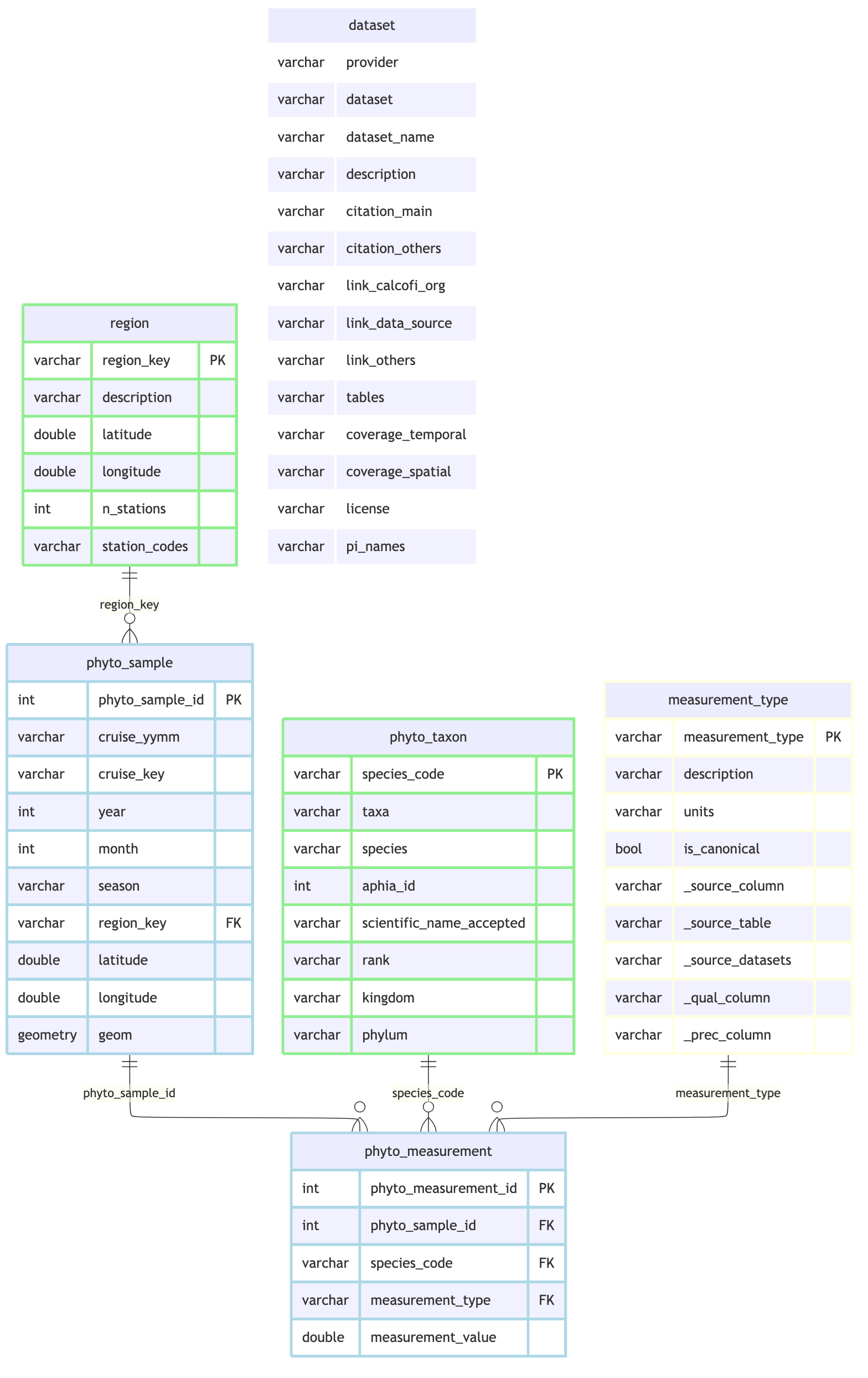
phyto_rels <- list(
  primary_keys = list(phyto_sample = "phyto_sample_id", phyto_measurement = "phyto_measurement_id",
                      phyto_taxon = "species_code", region = "region_key",
                      measurement_type = "measurement_type"),
  foreign_keys = list(
    list(table="phyto_sample",      column="region_key",       ref_table="region",           ref_column="region_key"),
    list(table="phyto_measurement", column="phyto_sample_id",  ref_table="phyto_sample",     ref_column="phyto_sample_id"),
    list(table="phyto_measurement", column="species_code",     ref_table="phyto_taxon",      ref_column="species_code"),
    list(table="phyto_measurement", column="measurement_type", ref_table="measurement_type", ref_column="measurement_type")))
cc_erd(con, tables = c("phyto_sample","phyto_measurement","phyto_taxon","region","measurement_type","dataset"),
       rels = phyto_rels,
       colors = list(lightblue = c("phyto_sample","phyto_measurement"),
                     lightgreen = c("phyto_taxon","region"),
                     lightyellow = "measurement_type", white = "dataset"))
# the SOURCE shape above documents the wrangling; relationships.json is written
# with the parquet outputs below, from core_relationships().

results <- validate_for_release(con, checks = "all", strict = FALSE)
cat("Validation:", ifelse(results$passed, "PASSED", "FAILED"), "\n")
dir_create(dir_parquet)
tbls_out <- core_output_tables(con, extra = c("region", "measurement_type", "dataset"))
write_parquet_outputs(con = con, output_dir = dir_parquet,
  tables = tbls_out,
  sort_by = list(obs = c("cruise_key", "measurement_type")), strip_provenance = FALSE)
build_relationships_json(rels = core_relationships(tbls_out), output_dir = dir_parquet,
  provider = provider, dataset = dataset)
d_tbls_rd <- read_csv(here("metadata/calcofi/phytoplankton/tbls_redefine.csv"))
d_flds_rd <- read_csv(here("metadata/calcofi/phytoplankton/flds_redefine.csv"))
build_metadata_json(con = con, d_tbls_rd = d_tbls_rd, d_flds_rd = d_flds_rd,
  metadata_derived_csv = c(here("metadata/core_dictionary.csv"),
                           here("metadata/calcofi/phytoplankton/metadata_derived.csv")),
  output_dir = dir_parquet, tables = tbls_out,
  set_comments = TRUE, provider = provider, dataset = dataset,
  workflow_url = cc$workflow_url, tables_owned = tables_owned)
if (Sys.getenv("CALCOFI_SKIP_GCS") == "") {
  sync_to_gcs(local_dir = dir_stage, sidecar_dir = dir_parquet, gcs_prefix = glue("ingest/{dir_label}"), bucket = "calcofi-db")
} else cat("CALCOFI_SKIP_GCS set - skipping the upload (local verification run)\n")
```
## Questions for Data Providers
```{r}
#| label: provider-questions
# one validated read + render for every ingest: the vocabulary and the column
# order live in calcofi4db, not in 16 hand-written factor() calls
questions_datatable(
  here(cc$questions_file),
  caption = "Questions for the CalCOFI phytoplankton data providers (ranked)")
```
```{r}
#| label: cleanup
close_duckdb(con); cat(glue("Parquet outputs written to: {dir_parquet}"), "\n")
```