---
title: "Interpolate Larvae"
author: "Ben Best"
format:
html:
toc: true
toc-depth: 3
code-fold: true
editor_options:
chunk_output_type: console
---
## CalCOFI Larvae
Constraints described by Andrew Thompson in CalCOFI Analysis for CINMS/MBNMS infographics ([calcofi.io/larvae-cinms](https://calcofi.io/larvae-cinms)):
- select only starboard samples from the bongo nets\
`net2cruise.netside = 'S'` (Port is usually ethanol sample vs formalin)
- select a minimum date\
`net2cruise.cruise_ymd >= '19780101'` \
diff't gear type, like oblique tow. internal table for
Questions:
- Should we limit (or have option) to filter by `linestation_core`?
- Should we limit (or have option) to limit by towtype?
```r
tbl(con, "net2cruise") |> pull(towtype) |> table()
```
```
     C1     CB     CV     MT     PV
 28,640 18,819  6,402 12,757 12,065
```
See `tow_types` table:
- CB: standard bongo tow starting 1978-01-01
- C1: previously used ringnet
### Species Groups
```{r larvae}
librarian::shelf(
  calcofi/calcofi4r,
  dplyr, DT, dygraphs, glue, here, mapview, purrr, readr, sf, tidyr,
  quiet = T)

source(here("../apps_dev/libs/db.R")) # con: database connection

tbl(con, "species_groups") |>
  group_by(spp_group) |>
  summarize(n_spp = n()) |>
  collect() |>
  datatable()
```
### Anchovy by Year-Month
```{r larvae-anchovy-ym}
spp_group <- "Anchovy"
ym        <- "2005-04"

monthly_csv <- here(glue("data/larvae_{spp_group}-ym.csv"))
ym_geo      <- here(glue("data/larvae_{spp_group}-{ym}.geojson"))

if (any(!file.exists(c(monthly_csv, ym_geo)))){
  d <- tbl(con, "net2cruise") |> # colnames() |> paste(collapse=", ")
    # netid, cruise_id, cruise_ymd, ship, line, stationid, station, latitude, longitude, orderocc, gebco_depth, netside, townumber, towtype, volsampled, shf, propsorted, starttime, geom
    filter(
      netside    == "S",
      cruise_ymd >= "19780101") |>
    left_join(
      tbl(con, "larvae_species"),
      # netid, spccode, scientific_name, common_name, larvaecount, itis_tsn
      by="netid") |>
    left_join(
      tbl(con, "species_groups") |>
        # spp_group, spccode
        filter(spp_group == !!spp_group),
      by="spccode") |>
    select(
      netid, longitude, latitude, starttime, volsampled,             # net2cruise
      spccode, scientific_name, common_name, larvaecount, itis_tsn,  # larvae_species
      spp_group) |>                                                  # species_groups
    arrange(starttime) |>
    collect() |> # 27,721 × 6 <-  145,724 × 11
    group_by(
      netid, longitude, latitude, starttime, volsampled) |>
    nest() |>
    mutate(
      larvaecount = map_int(data, \(x){
        x |>
          filter(
            !is.na(spp_group)) |>
          summarize(
            n = sum(larvaecount, na.rm = T)) |>
          pull(n) } ) )

  d_monthly <- d |>
    select(-data) |>
    mutate(
      ym_chr = format(starttime, "%Y-%m"),
      ym     = glue("{ym_chr}-01") |> as.Date()) |>
    group_by(ym) |>
    summarize(
      vol = first(volsampled),
      n   = sum(larvaecount)) |>
    mutate(
      n_log10         = log10(n + 0.001),
      n_per_vol       = n / vol,
      n_per_vol_log10 = log10(n_per_vol + 0.0001))
  write_csv(d_monthly, monthly_csv)

  pts_ym <- d |>  # 99 × 7 <- 27,721 × 7
    filter(
      format(starttime, "%Y-%m") == "2005-04") |>
    select(-data) |>
    rename(
      n   = larvaecount,
      vol = volsampled) |>
    mutate(
      n_log10         = log10(n + 0.001),
      n_per_vol       = n / vol,
      n_per_vol_log10 = log10(n_per_vol + 0.0001)) |>
    sf::st_as_sf(
      coords = c("longitude", "latitude"),
      crs    = 4326,
      remove = F)
  write_sf(pts_ym, ym_geo, delete_dsn = T)
}

d_monthly <- read_csv(monthly_csv, show_col_types = F)

d_monthly |>
  select(ym, n_per_vol) |>
  arrange(ym) |>
  dygraph(
    x = "ym",
    y = "n_per_vol",
    main = glue("Larvae Counts by Month for {spp_group}"))
```
### Map of Anchovy Larvae on 2005-04
```{r anchovy-map-2005-04}
pts_ym <- read_sf(ym_geo)

mapView(
  pts_ym,
  zcol        = "n_per_vol_log10",
  col.regions = rev(RColorBrewer::brewer.pal(11,"Spectral")))
```
## Copernicus Marine
- [Global Ocean Physics Reanalysis | Copernicus Marine Service](https://data.marine.copernicus.eu/product/GLOBAL_MULTIYEAR_PHY_001_030/description)
> The GLORYS12V1 product is the CMEMS global ocean eddy-resolving (1/12° horizontal resolution, 50 vertical levels) reanalysis covering the altimetry (1993 onward)...
> This product includes daily and monthly mean files for temperature, salinity, currents, sea level, mixed layer depth and ice parameters from the top to the bottom. The global ocean output files are displayed on a standard regular grid at 1/12° (approximatively 8 km) and on 50 standard levels.
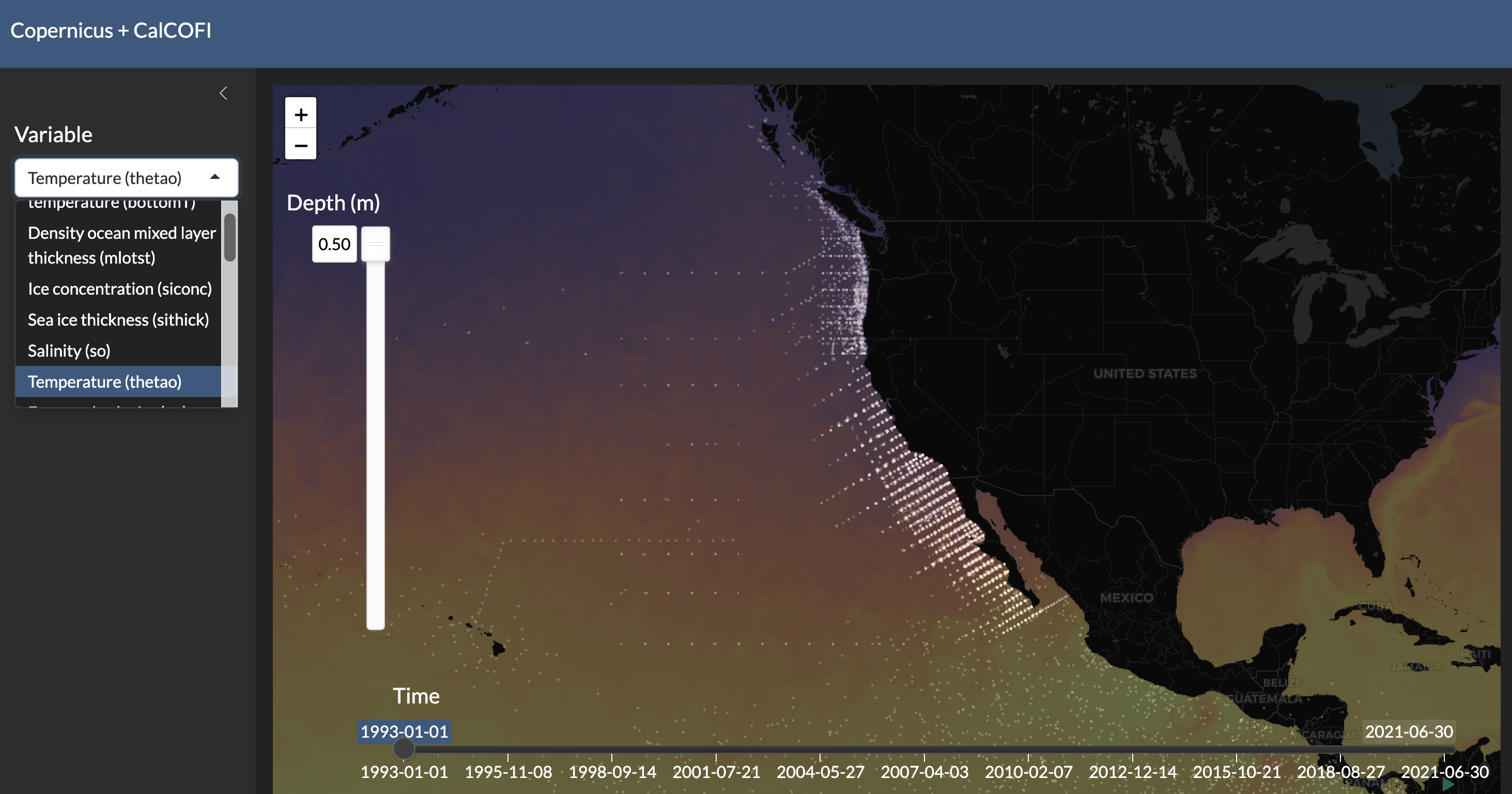
### Visualizing Copernicus in 4D (lon, lat, depth, time)
The Web Map Tile Service (WMTS) allows for interactive map rendering by `variable`, `time` and `depth`. It does not include the raw data values, so is ony for visualization.
The [WMTS `GetCapabilities`](https://wmts.marine.copernicus.eu/teroWmts/GLOBAL_MULTIYEAR_PHY_001_030?request=GetCapabilities) gets parsed to collect available variables, depths (`elevation`) and dates (`time`) for the given `product_id/dataset_id/variable`.
See:
- code: [github.com/CalCOFI/apps:copernicus/](https://github.com/CalCOFI/apps/tree/main/copernicus)
- app: [shiny.calcofi.io/copernicus](https://shiny.calcofi.io/copernicus/)
### Subset raster of surface temperature for 2005-04
Using the CLI.
```{r cm-setup}
librarian::shelf(
  glue, httr2, leaflet, lubridate, xml2)

# Global Ocean Physics Reanalysis
#   1993-01-01 to 2021-06-01
product_id = "GLOBAL_MULTIYEAR_PHY_001_030"
# dataset_id = "cmems_mod_glo_phy_my_0.083deg_P1D-m" # P1D: daily
dataset_id = "cmems_mod_glo_phy_my_0.083deg_P1M-m" # P1M: monthly

# Global Ocean Physics Analysis and Forecast
#   1 Nov 2020 to 31 May 2024
# product_id = "GLOBAL_ANALYSISFORECAST_PHY_001_024"
# dataset_id = "cmems_mod_glo_phy-thetao_anfc_0.083deg_P1M-m"

# my:    MY (Multi-Year/Reprocessed)
# myint: MY interim (MYINT)
# nrt:   NRT (Near Real Time)

variable = "thetao"
date     = as.Date("2005-04-01") |> as.POSIXct()
```
- `product_id`: `r product_id`
- `dataset_id`: `r dataset_id`
- `variable`: `r variable` (temperature)
```{r cm-cc}
librarian::shelf(
  calcofi/calcofi4r,
  dplyr, glue, here, jsonlite, leaflet, lubridate, mapview, purrr, sf, terra,
  tibble, tidyr)

cm   = "/opt/homebrew/Caskroom/mambaforge/base/envs/copernicusmarine/bin/copernicusmarine"
user = "bbest1"
# pass = readLines("~/My Drive/private/data.marine.copernicus.eu_bbest1-password.txt")
pass = "temporary"
verbose = F

# CalCOFI bounding box
b <- st_union(cc_grid_zones) |> st_bbox()
# b
#       xmin       ymin       xmax       ymax
# -135.23008   18.42757 -105.77692   49.23891

m_json <- here(glue("data/copernicusmarine/{dataset_id}.json"))
cmd <- glue("{cm} describe --include-datasets -c {dataset_id}")
if (!file.exists(m_json))
  system(cmd, intern = TRUE) |> writeLines(m_json)
m_o <- read_json(m_json)
# listviewer::jsonedit(m_o)

get_coord = function(o, v){
  if (!v %in% names(o))
    return(NA)
  if (length(o[[v]]) == 0)
    return(NA)
  o[[v]] |>
    as.character()
}

coord_date <- function(df, col){

  df |>
    filter(coord_id == "time") |>
    pull(!!col) |>
    (\(x) as.double(x) / 1000)() |>
    as_datetime(origin = "1970-01-01", tz = "UTC") |>
    as_date()
}

m_vars <- m_o |>
  pluck("products", 1, "datasets", 1, "versions", 1, "parts", 1, "services") |>
  keep(\(x) x$service_type$service_name == "arco-geo-series") |>
  pluck(1, "variables")

d_vars_coords <- m_vars %>%
  tibble(
    short_name    = map_chr(., "short_name"),
    standard_name = map_chr(., "standard_name"),
    units         = map_chr(., "units"),
    coord         = map(., "coordinates") ) |>
  select(-`.`) |>
  unnest(coord) |>
  mutate(
    coord_id            = map_chr(coord, "coordinates_id"),
    coord_units         = map_chr(coord, "units"),
    coord_min_val       = map_chr(coord, get_coord, "minimum_value"),
    coord_max_val       = map_chr(coord, get_coord, "maximum_value"),
    coord_step          = map_chr(coord, get_coord, "step"),
    coord_chunk_length  = map_chr(coord, get_coord, "chunking_length"),
    coord_chunk_type    = map_chr(coord, get_coord, "chunk_type"),
    coord_chunk_ref     = map_chr(coord, get_coord, "chunk_reference_coordinate"),
    coord_chunk_geo     = map_chr(coord, get_coord, "chunk_geometric_factor"),
    coord_values        = map(coord, "values"),
    coord_values_n      = map_int(coord_values, length))
#
# d_vars_coords |> select(short_name, coord_id) |> table()
#           coord_id
# short_name depth latitude longitude time
#    bottomT     1        1         1    1
#    mlotst      1        1         1    1
#    siconc      1        1         1    1
#    sithick     1        1         1    1
#    so          1        1         1    1
#    thetao      1        1         1    1
#    uo          1        1         1    1
#    usi         1        1         1    1
#    vo          1        1         1    1
#    vsi         1        1         1    1
#    zos         1        1         1    1
#
# d_vars_coords |> select(coord_id, coord_values_n) |> table()
#            coord_values_n
# coord_id     0 50
#   depth      0 11
#   latitude  11  0
#   longitude 11  0
#   time      11  0

d_vars <- d_vars_coords |>
  nest(.by = c(short_name, standard_name, units)) |>
  mutate(
    date_min = map_dbl(data, coord_date, "coord_min_val") |>
      as.Date(),
    date_max = map_dbl(data, coord_date, "coord_max_val") |>
      as.Date())

depths <- d_vars |>
  filter(
    short_name == "thetao") |>
  pull(data) |>
  (\(x) x[[1]])() |>
  filter(
    coord_id == "depth") |>
  pull(coord_values) |>
  unlist()

# depths <- obj$products[[1]]$datasets[[1]]$versions[[1]]$parts[[1]]$services[[2]]$variables[[1]]$coordinates[[4]][["values"]] |>
#   unlist()
depth <- depths[length(depths)] * -1

# output filename
nc <- here(glue("data/copernicusmarine/{dataset_id}__{variable}__{date}.nc"))

# https://help.marine.copernicus.eu/en/articles/7970514-copernicus-marine-toolbox-installation
# mamba update --name copernicusmarine copernicusmarine --yes
# copernicusmarine, version 1.2.2
cmd <- glue("
  {cm} subset -i {dataset_id} \\
  -x {b$xmin} -X {b$xmax}     \\
  -y {b$ymin} -Y {b$ymax}     \\
  -t {date}   -T {date + months(1) - days(1)}       \\
  -z {depth - 0.01}  -Z {depth +  - 0.01}      \\
  -v {variable}               \\
  -o {dirname(nc)} -f {basename(nc)} \\
  --username {user} --password '{pass}' \\
  --force-download")
if (verbose)
  print(cmd)
if (!file.exists(nc))
  system(cmd, intern = TRUE)

r <- rast(nc)
# dimensions  : 369, 353, 1  (nrow, ncol, nlyr)
# resolution  : 0.08333334, 0.08333334  (x, y)
# extent      : -135.2083, -105.7917, 18.45833, 49.20833  (xmin, xmax, ymin, ymax)
r_3857 <- leaflet::projectRasterForLeaflet(r, method = "bilinear")
# dimensions  : 403, 313, 1  (nrow, ncol, nlyr)
# resolution  : 10458.57, 10458.57  (x, y)

plet(r_3857, tiles = "Esri.WorldImagery")
```
## Interpolate larvae on Copernicus grid
### IDW(x,y)
```{r cm-larvae-idw}
# basename(nc) # cmems_mod_glo_phy_my_0.083deg_P1M-m__thetao__2022-04-01.nc"

r_cm <- rast(nc)

r_idw <- terra::interpIDW(
  x = r_cm,
  y = pts_ym |> terra::vect(),
  "n_per_vol_log10",
  # borrow from defaults in [calcofi4r:: pts_to_rast_idw()](https://github.com/CalCOFI/calcofi4r/blob/5e9508565a78785f8b374c3b8b5e2c4cdf559ed0/R/analyze.R#L236C5-L236C100)
  radius = 1.5, power = 1.3, smooth = 0.2,
  maxPoints = Inf, minPoints = 1, near = F, fill = NA) |>
  mask(r_cm)
names(r_idw)     <- "n_per_vol_log10_idw"
# time(r_idw) # "2005-04-01 UTC"
varnames(r_idw)  <- ""
longnames(r_idw) <- ""
# units(r_idw) ""
# plot(r_idw)

pts_ymi <- r_idw |>
  terra::extract(pts_ym, method = "simple", bind = T) |>
  st_as_sf() |>
  mutate(
    dif_idw = n_per_vol_log10 - n_per_vol_log10_idw)

# pts_ymi$dif_idw |> summary()
#     Min.  1st Qu.   Median     Mean  3rd Qu.     Max.     NA's
# -2.24324 -0.28024  0.00000  0.01276  0.38674  1.76034        6

d_mi <- pts_ymi |>
  st_drop_geometry() |>
  filter(!is.na(n_per_vol_log10_idw))

rmse_idw <- with(
  d_mi,
  sqrt(
    sum((n_per_vol_log10_idw - n_per_vol_log10)^2) /
      nrow(d_mi) ) )
# [1] 0.7824212

mapView(
  r_idw,
  zcol        = "n_per_vol_log10_idw",
  col.regions = rev(RColorBrewer::brewer.pal(11,"Spectral"))) +
mapView(
  pts_ymi,
  zcol        = "n_per_vol_log10",
  col.regions = rev(RColorBrewer::brewer.pal(11,"Spectral"))) +
mapView(
  pts_ymi,
  zcol        = "dif_idw",
  col.regions = rev(RColorBrewer::brewer.pal(11,"Spectral")))
```
Root Mean Square Error: `r rmse_idw`
### GAM(x, y)
```{r cm-larvae-gam-xy}
librarian::shelf(mgcv)

# fit GAM
mdl_xy <- mgcv::gam(
  n_per_vol_log10 ~ s(longitude, latitude, k = 60),
  data   = pts_ymi |> st_drop_geometry() |>
    select(n_per_vol_log10, longitude, latitude),
  method = "GCV.Cp", # method = "REML",
  family = gaussian())
# summary(mdl_xy)
# Family: gaussian
# Link function: identity
#
# Formula:
# n_per_vol_log10 ~ s(longitude, latitude, k = 60)
#
# Parametric coefficients:
#             Estimate Std. Error t value Pr(>|t|)
# (Intercept)  0.25360    0.06438   3.939 0.000117 ***
# ---
# Signif. codes:  0 ‘***’ 0.001 ‘**’ 0.01 ‘*’ 0.05 ‘.’ 0.1 ‘ ’ 1
#
# Approximate significance of smooth terms:
#                         edf Ref.df     F p-value
# s(longitude,latitude) 12.91  18.26 11.79  <2e-16 ***
# ---
# Signif. codes:  0 ‘***’ 0.001 ‘**’ 0.01 ‘*’ 0.05 ‘.’ 0.1 ‘ ’ 1
#
# R-sq.(adj) =  0.526   Deviance explained = 55.7%
# GCV = 0.86605  Scale est. = 0.80397   n = 194

p_idw <- r_idw |>
  as.points() |>
  st_as_sf() |>
  mutate(
    longitude = sf::st_coordinates(geometry)[,1],
    latitude  = sf::st_coordinates(geometry)[,2])

# range(p_idw$n_per_vol_log10_idw)
# [1] -1.000000  2.413467

# predict with GAM
p_idw$n_per_vol_log10_xy <- predict.gam(
  mdl_xy,
  newdata = p_idw |>
    st_drop_geometry() |>
    select(longitude, latitude),
  type = "response") # link") # "response")
# range(p_idw$n_per_vol_log10_xy) # -4.334638  0.183662

r_xy <- rasterize(
  p_idw |>
    st_drop_geometry() |>
    select(longitude, latitude) |>
    as.matrix(),
  r_idw,
  values = p_idw$n_per_vol_log10_xy)
# range(values(r_xy, na.rm=T)) # -4.334638  0.183662
# plot(r_xy)
names(r_xy)     <- "n_per_vol_log10_xy"

pts_ymix <- r_xy |>
  terra::extract(pts_ymi, method = "simple", bind = T) |>
  st_as_sf() |>
  mutate(
    dif_xy = n_per_vol_log10 - n_per_vol_log10_xy)

# pts_ymix$dif_xy |> summary()
#      Min.   1st Qu.    Median      Mean   3rd Qu.      Max.      NA's
# -2.259856 -0.326382 -0.000841  0.024003  0.401710  2.446836         6

d_mix <- pts_ymix |>
  st_drop_geometry() |>
  filter(!is.na(n_per_vol_log10_idw))

rmse_xy <- with(
  d_mix,
  sqrt(
    sum((n_per_vol_log10_xy - n_per_vol_log10)^2) /
      nrow(d_mix) ) )
# [1] 0.8445961

mapView(
  r_xy,
  zcol        = "n_per_vol_log10_xy",
  col.regions = rev(RColorBrewer::brewer.pal(11,"Spectral"))) +
mapView(
  pts_ymix,
  zcol        = "n_per_vol_log10",
  col.regions = rev(RColorBrewer::brewer.pal(11,"Spectral"))) +
mapView(
  pts_ymix,
  zcol        = "dif_xy",
  col.regions = rev(RColorBrewer::brewer.pal(11,"Spectral")))
```
Root Mean Square Error: `r rmse_xy`
### GAM(x, y, temperature)
```{r cm-larvae-gam-xyt}
librarian::shelf(mgcv)

names(r_cm) <- "thetao"

pts_ymixt <- r_cm |>
  terra::extract(pts_ymix, method = "simple", bind = T) |>
  st_as_sf()

# fit GAM
mdl_xyt <- mgcv::gam(
  n_per_vol_log10 ~ s(longitude, latitude, k = 60) + s(thetao),
  data   = pts_ymixt |> st_drop_geometry() |>
    select(n_per_vol_log10, longitude, latitude, thetao),
  method = "GCV.Cp", # method = "REML",
  family = gaussian())
# summary(mdl_xyt)
# Family: gaussian
# Link function: identity
#
# Formula:
# n_per_vol_log10 ~ s(longitude, latitude, k = 60) + s(thetao)
#
# Parametric coefficients:
#             Estimate Std. Error t value Pr(>|t|)
# (Intercept)  0.25181    0.06219   4.049 7.84e-05 ***
# ---
# Signif. codes:  0 ‘***’ 0.001 ‘**’ 0.01 ‘*’ 0.05 ‘.’ 0.1 ‘ ’ 1
#
# Approximate significance of smooth terms:
#                          edf Ref.df      F p-value
# s(longitude,latitude) 12.767 18.199 12.505  <2e-16 ***
# s(thetao)              6.151  7.214  1.556   0.146
# ---
# Signif. codes:  0 ‘***’ 0.001 ‘**’ 0.01 ‘*’ 0.05 ‘.’ 0.1 ‘ ’ 1
#
# R-sq.(adj) =  0.576   Deviance explained = 61.9%
# GCV = 0.81327  Scale est. = 0.7271    n = 188

p_cm <- r_cm |>
  mask(r_idw) |>
  trim() |>
  as.points() |>
  st_as_sf() |>
  mutate(
    longitude = sf::st_coordinates(geometry)[,1],
    latitude  = sf::st_coordinates(geometry)[,2])

# range(p_idw$n_per_vol_log10_idw)
# [1] -1.000000  2.413467

# predict with GAM
p_cm$n_per_vol_log10_xyt <- predict.gam(
  mdl_xyt,
  newdata = p_cm |>
    st_drop_geometry() |>
    select(longitude, latitude, thetao),
  type = "response") # link") # "response")
# range(p_cm$n_per_vol_log10_xyt) # -5.369945  1.165597

r_xyt <- rasterize(
  p_cm |>
    st_drop_geometry() |>
    select(longitude, latitude) |>
    as.matrix(),
  r_idw,
  values = p_cm$n_per_vol_log10_xyt)
# range(values(r_xyt, na.rm=T)) # -5.369945  1.165597
# plot(r_xy)
names(r_xyt)     <- "n_per_vol_log10_xyt"

pts_ymixt <- r_xyt |>
  terra::extract(pts_ymixt, method = "simple", bind = T) |>
  st_as_sf() |>
  mutate(
    dif_xyt = n_per_vol_log10 - n_per_vol_log10_xyt)

# pts_ymixt$dif_xyt |> summary()
#      Min.   1st Qu.    Median      Mean   3rd Qu.      Max.      NA's
# -3.596383 -0.429587 -0.003567  0.002183  0.587119  2.562442         6


d_mixt <- pts_ymixt |>
  st_drop_geometry() |>
  filter(!is.na(n_per_vol_log10_idw))

rmse_xyt <- with(
  d_mixt,
  sqrt(
    sum((n_per_vol_log10_xyt - n_per_vol_log10)^2) /
      nrow(d_mixt) ) )
# rmse_xyt
# [1] 0.8054934

mapView(
  r_xyt,
  zcol        = "n_per_vol_log10_xyt",
  col.regions = rev(RColorBrewer::brewer.pal(11,"Spectral"))) +
mapView(
  pts_ymixt,
  zcol        = "n_per_vol_log10",
  col.regions = rev(RColorBrewer::brewer.pal(11,"Spectral"))) +
mapView(
  pts_ymixt,
  zcol        = "dif_xyt",
  col.regions = rev(RColorBrewer::brewer.pal(11,"Spectral")))
```
Root Mean Square Error: `r rmse_xyt`
