1 Load R packages, connect to remote duckdb database
Load R packages. Note that the librarian package is used to manage package dependencies, and it will install any missing packages automatically.
We can’t directly load a remote duckdb database, so we will attach it to a local duckdb connection. The remote database is hosted on CalCOFI’s file server.
We will use the duckdb community h3 extension to generate the hexagon polygons.
if (!requireNamespace("librarian", quietly =TRUE)) {install.packages("librarian")}librarian::shelf( DBI, dplyr, DT, duckdb, glue, here, leaflet.extras, mapview, sf, tibble, tidyr,quiet = T)mapviewOptions(basemaps ="Esri.OceanBasemap",vector.palette = \(n) hcl.colors(n, palette ="Spectral"))url_dk <-"https://file.calcofi.io/calcofi.duckdb"tmp_dk <-here("data/tmp.duckdb")con <-dbConnect(duckdb(), dbdir = tmp_dk)res <-dbExecute(con, "INSTALL h3 FROM community; LOAD h3;")res <-dbExecute(con, glue("ATTACH IF NOT EXISTS '{url_dk}' AS calcofi; USE calcofi"))
Note that since the ATTACH statement above uses a URL, duckdb implicitly installs and loads the httpfs extension, which allows duckdb to read from remote files over HTTP(S).
2 Explore db structure
Use a couple DBI functions to explore the database structure and list tables and fields in a table.
Note that you might need to sometimes restart your R session (under Session menu in RStudio) to connect to the local duckdb.
6 Next steps
Here are some potential next steps that come to mind – please feel free to come up with your own:
Source Code
---title: "Explore using the remote CalCOFI duckdb to generate hexagonal summaries"editor_options: chunk_output_type: console---## Load R packages, connect to remote duckdb databaseLoad R packages. Note that the `librarian` package is used to manage package dependencies, and it will install any missing packages automatically.We can't directly load a remote duckdb database, so we will attach it to a local duckdb connection. The remote database is hosted on [CalCOFI's file server](https://file.calcofi.io/).We will use the duckdb community [h3 extension](https://duckdb.org/community_extensions/extensions/h3.html) to generate the hexagon polygons.To see how the resolutions of hexagons vary, see:- [Tables of Cell Statistics Across Resolutions | H3](https://h3geo.org/docs/core-library/restable/#edge-lengths)```{r setup}if (!requireNamespace("librarian", quietly =TRUE)) {install.packages("librarian")}librarian::shelf( DBI, dplyr, DT, duckdb, glue, here, leaflet.extras, mapview, sf, tibble, tidyr,quiet = T)mapviewOptions(basemaps ="Esri.OceanBasemap",vector.palette = \(n) hcl.colors(n, palette ="Spectral"))url_dk <-"https://file.calcofi.io/calcofi.duckdb"tmp_dk <-here("data/tmp.duckdb")con <-dbConnect(duckdb(), dbdir = tmp_dk)res <-dbExecute(con, "INSTALL h3 FROM community; LOAD h3;")res <-dbExecute(con, glue("ATTACH IF NOT EXISTS '{url_dk}' AS calcofi; USE calcofi"))```Note that since the `ATTACH` statement above uses a URL, duckdb implicitly installs and loads the [`httpfs`](https://duckdb.org/docs/stable/core_extensions/httpfs/overview.html) extension, which allows duckdb to read from remote files over HTTP(S).## Explore db structureUse a couple [`DBI`](https://dbi.r-dbi.org/) functions to explore the database structure and list tables and fields in a table.```{r con_dbi}dbListTables(con)dbListFields(con, "site")```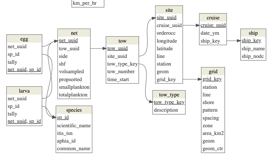{#fig-schema}## Explore `larva` observations by `species````{r}d_sp_n <-tbl(con, "species") |>left_join(tbl(con, "larva"),by ="sp_id") |>group_by(sp_id, scientific_name, common_name) |>summarize(n =n(),.groups ="drop") |>arrange(desc(n)) |>collect()datatable(d_sp_n)```## Map anchovy observations by hexagon```{r fig-hex_sp}#| fig-cap: "Map of Northern anchovy larval counts by hexagon (H3 resolution 3)."sp_common <-"Northern anchovy"hex_res <-4# 1:10hex_fld <-glue("hex_h3_res{hex_res}")hex_sp <-tbl(con, "species") |>filter(common_name ==!!sp_common) |>left_join(tbl(con, "larva"),by ="sp_id") |>left_join(tbl(con, "net"),by ="net_uuid") |>left_join(tbl(con, "tow"),by ="tow_uuid") |>left_join(tbl(con, "site"),by ="site_uuid") |>rename(hex_int = .data[[hex_fld]]) |>group_by(hex_int) |>summarize(value =sum(tally),.groups ="drop") |>mutate(hex_id =sql("HEX(hex_int)")) |>mutate(hex_wkt =sql("h3_cell_to_boundary_wkt(hex_id)")) |>select(hexid = hex_id, value, hex_wkt) |>collect() |>st_as_sf(wkt ="hex_wkt", crs =4326)mapView(hex_sp, zcol ="value", layer.name = sp_common) |>removeMapJunk(c("layersControl", "homeButton")) |>addFullscreenControl()```## Close db connection```{r cleanup_con_dk}dbDisconnect(con, shutdown = T); duckdb_shutdown(duckdb()); rm(con)```Note that you might need to sometimes restart your R session (under Session menu in RStudio) to connect to the local duckdb.## Next stepsHere are some potential next steps that come to mind -- please feel free to come up with your own:- [ ] Convert the above code into a data retrieval function that accepts `species_common` (or `species_scientific`) and `hex_res` as arguments.- [ ] Write another helper function to map the hexagons.- [ ] Make a Shiny app with map output from selected drop-downs of species and hexagon resolution.- [ ] Expand filtering function to include `depth`, `season`, etc., a la the [oceano](https://shiny.calcofi.io/oceano) and [taxa](https://shiny.calcofi.io/taxa-dev) apps
